Analysis and Optimization of a Spatial Parallel Mechanism for a New 5-DOF Hybrid Serial-Parallel Manipulator

Abstract

Hybrid manipulators have potentially application in machining industries and attract extensive attention from many researchers on the basis of high stiffness and high dexterity. Therefore, in order to expand the application prospects of hybrid manipulator, a novel 5-degree-of-freedom (DOF) hybrid serial-parallel manipulator (HSPM) is proposed. Firstly, the design plan of this manipulator is introduced. Secondly, the analysis of this manipulator is carried out in detail, including kinematics analysis, statics analysis, and workspace analysis. Especially, an amplitude equivalent method of disposing the over-constrained force/couple to the non-overconstrained force/couple is used in the statics analysis. Then, three performance indices are used to optimize the PM. Two of them have been widely used, and the third one is a new index which considers the characteristics of the actuated force. Based on the performance indices, the performance atlas is drawn and the optimal design of the PM is investigated. In order to satisfy the anticipant kinetic characteristics of the PM, the verification of the optimized physical dimension is done and the workspace based on the optimized physical dimension is carried out. This paper will lay good theoretical foundations for application of this novel HSPM and also can be applied to other hybrid manipulators.

1 Introduction

Since the appearance of parallel mechanisms (PMs), PMs have been studied widely, mainly because of PMs owning the characteristics of compact structure, high stiffness, and high load capacity compared with serial mechanisms [1, 2]. In the early stage, Klaus Cappel developed the first flight simulator, which was based on a 6-degree-of-freedom (DOF) Gough-Stewart platform. Hereafter, this device has been widely used in the fields of flight simulator, medical treatment, and communication. Then, as the application extension of PMs, the lower-mobility (two to five DOFs) PMs appeared. The lower-mobility PMs have become a research hotspot due to their desirable characteristics, such as simple structure, low kinematic coupling, low cost, and easy control [3,4,5]. For instance, Xie et al. [3], Huang et al. [4] and Joshi et al. [5] researched the type synthesis for different types of lower-mobility PM. Clavel et al. [6], invented the 3-DOF robot DELTA, which was a successful application case of the lower-mobility PMs. Except that, one of the most important lower-mobility PMs is the PM with one translational DOF and two rotational DOFs (2R1T): the 3RPS PM analyzed by Zhang et al. [7], is a typical 2R1T PM (R, P, and S stand for revolute, prismatic, and spherical joints, respectively). Actually, the 2R1T PMs have different properties about their rotational axes. Huang, et al. [8] analyzed the motion characteristics of rotational axis. For the two rotational DOFs of 2R1T PMs, the rotational axes of PMs can be divided into two types: continuous rotational axis (CRA) and instantaneous rotational axis (IRA). Here, CRA/IRA (continuous rotational axis) represents rotation axis. For the CRA, the moving platform (MP) can rotate around the rotation axis continually. For the IRA, the MP can only rotate around the rotational axis in a specific pose [9]. Compared with the general 2R1T PMs, the 2R1T PMs with two CRAs are easier to implement trajectory planning, parameter calibration, and motion control, which allows for a variety of application prospects. Nevertheless, there are only a few types of 2R1T PMs with two CRAs, which has limited the development and engineering application of this kind of mechanism.

In the processing industry, most of the complex space surfaces (such as the surfaces of engine blade, propeller blade, and nuclear evaporator head) need five-axis simultaneous machining center. Consequently, using the five or six DOFs PMs is an appropriate choice, but the multi-DOF PMs are composed of multi-hinge and multi-chain. Under the influence of the complicated self-structure, the orientation capability of multi-DOF PMs is limited. And the high kinematic coupling, complicated dynamics model, hard control also should be noted. Taking these disadvantages into account, the structure of machines should be improved. Therefore, the hybrid serial-parallel manipulators (HSPMs) based on the 2R1T PMs may be a trend, which present a compromise between the high stiffness of PMs and the good flexibility, large workspace of serial mechanisms [10, 11]. For example, the 5-axis FSW proposed by Li [12], is installed by concatenating a 2-DOF PP serial mechanism on the 2R1T PM 2SPR/RPS. The Tricept [13], Trivariant 5-DOF HSPM [14] and Exechon five-axis machining center [15] are constructed by concatenating the 2-DOF sway heads on the MPs of the 2R1T PMs: 3UPS/UP, 2UPS/UP, and 2UPR/SPR, respectively (U stands for universal joints).

Except for the configuration properties of PMs, optimal design is also a hot topic [16,17,18]. A successful optimization can effectively improve the motion/force transmission and orientation capability [19,20,21], etc. Ref. [19] mentioned that the condition number of Jacobian matrix and global condition index were not used to parallel robots with mixed types of DOFs. So for the 2R1T PMs with combined DOFs, the suggested indices [19, 22] are independent of any coordinate frame and more appropriate for HSPMs. Basically, the linear actuated unit of the above mentioned PMs is the ball screw system, the fluctuations of its friction moment will have a direct impact on the stationarity of the driving system. Generally speaking, the axial load has direct effect on friction moment. So the fluctuations of actuated force will affect the friction moment, and then affect mechanical motion properties and dynamic behavior in the practical application [23, 24]. Other than motion/force transmission and orientation capability indices, the stability of the actuated force in each limb also needs to be paid attention.

In this paper, a novel 5-DOF HSPM is introduced whose parallel part is an over-constrained lower mobility 2R1T PM. The remainder contents of this paper are organized as follows: In Section 2, the design plan and description of the 5-DOF HSPM is performed detailedly. In Section 3, the systematical analysis of this hybrid manipulator is carried out, including kinematics, statics and workspace analysis. Section 4 reports the dimensional optimization on the basis of three indices including transmission capacity, good orientation capability and force stability. Section 5 presents conclusions.

2 Novel Spatial 5-DOF HSPM

2.1 Design Plan of a New 5-DOF HSPM

The core part of the Exechon five-axis machining center is the 2UPR/SPR PM with ten single-DOF joints, so 2UPR/SPR PM has a high stiffness. On the basis of this reason, a 3-DOF 2RPU/UPR PM with nine single-DOF joints is used. Here, one point should be mentioned, the 2RPU/UPR PM in this paper is different from the 2RPU/UPR PM in Ref. [25]. Actually, the MP and the base of the PM are inverse, which is the same as the case of 3SPR and 3RPS PMs.

As shown in Figure 1, the 2RPU/UPR PM has two CRAs, one of these CRAs is close to the base (marked as r₁) and the other one distributes close to the MP (marked as r₂). The rotation around r₁-axis can make the MP from side to side along x₀-axis, which means the end effector can realize the extensive translational movement along x₀-axis. The rotation around r₂-axis is used to adjust the orientation of the MP at one direction. And two rotation DOFs can be accomplished independently. For example, the actuators in limb₁ and limb₃ are used to accomplish the rotation around r₁-axis; the actuator in limb₂ is used to accomplish the rotation around r₂-axis. Besides the two rotation DOFs, the translational DOF of this PM is along z₀-axis, which needs all of these three actuators coordinated movement. The single-DOF sway head on the MP is used to realize the orientation transformation at the other direction. The translational table on the base is used to realize the extensive translational movement along y₀-axis. So this novel 5-DOF HSPM can obtain both excellent positioning capability and greater rotation capability.

Figure 1

A 5-DOF HSPM

The 3D model of the spatial 5-DOF HSPM is shown as Figure 1(a), the schematic diagram is shown as Figure 1(b).

2.2 Configuration Description of the 5-DOF HSPM

As shown in Figure 1(b), features of the parallel part are as follows: the cross points of two axes within each U joint are denoted by A₂, a₁ and a₃ respectively; A₁ and A₃ are the projections of a₁ and a₃ onto the base along the direction of corresponding P joints; a₂ is the projection of A₂ onto the MP along the direction of P joint. The triangles a₁a₂a₃ and A₁A₂A₃ are isosceles and similar. The reference frame A: O-XYZ is attached to the base with X-axis pointing along vector OA₃ and Y-axis pointing along vector A₂O, where O is the midpoint of A₁A₃. The moving frame a: o-xyz is attached to the MP with x-axis pointing along vector oa₃ and y-axis pointing along vector a₂o, where o is the midpoint of a₁a₃.

Limb₁ and limb₃ are identical RPU limbs (P represents an actuated prismatic joint), which are restricted in the plane A₁A₃a₃a₁. Limb₂ is a UPR limb, which is restricted in the plane A₂a₂oO, and plane A₂a₂oO is always perpendicular to plane A₁A₃a₃a₁. For the two RPU limbs, the axes of R joints are parallel to plane defined by the axes of the U joints connected to the limbs and perpendicular to the plane A₁A₃a₃a₁. The translational direction of actuated P joints is perpendicular to the axes of R joints. The axes of two U joints connected to the MP are aligned. For the UPR limb, the axis of R joint is parallel to line a₁a₃. The axis of U joint connected to the base is parallel to the axes of R joints in limb₁ and limb₃. The translational direction of actuated P joint is perpendicular to the axis of R joint and the adjacent axis of U joint.

For the single-DOF sway head, its rotational axis is always parallel to line oa₂. For the translational table, its translational direction is along line OA₂.

3 Analysis of the Hybrid Manipulator

3.1 DOF Analysis of 2RPU/UPR PM

Below the revised Kutzbach-Grübler formula is used to calculate the DOF of 2RPU/UPR PM. The formula is shown as [26]

$$ M = d(n - g - 1) + \sum {f_{i} } + v - \zeta , $$

(1)

where M is the number of DOF, d is the rank of PM, n is the number of components, g is the number of joints, $\sum {f_{i} }$ is the sum of joints DOF, ν is the number of redundancy constraints, $\zeta$ is the number of isolated DOF.

According to the reciprocal screw theory [27], we know that every limb of 2RPU/UPR PM exists a constraint force and a constraint couple. In each limb, the constraint force passes through the U joint and is parallel to the axis of R joint; and the constraint couple is perpendicular to all of the rotational axes. Therefore, the direction of constraint couples is identical, in other words, this PM has one common constraint.

As the relationships among these joints are invariable at arbitrarily instantaneous pose of this PM, the constraint force/couple are all conform to the above analysis. Then, the parameters in Eq. (1) can be obtained as d = 6 − λ =5 (λ is the number of common constraint), $n = 8,$ $g = 9,$ $\sum {f_{i} } = 12,$ $v = 1,$ $\zeta = 0.$ Substituting the above parameters into Eq. (1), the DOF of PM is obtained: $M = 3.$ As for these three DOFs, the translational DOF is along Z-axis. One of the rotational DOFs is around Y-axis; the other one is around x-axis. It should be noted that the Y-axis is r₁-axis and the x-axis is r₂-axis, both of them are CRAs.

3.2 Inverse Kinematics Analysis of 2RPU/UPR PM

Simple inverse kinematics is good for machine control, so it is necessary to solve the inverse kinematics of PMs. As it is known, the inverse kinematics of PMs is simple, especially for 2R1T PMs. Thus, the solving process will be relatively easy, and only some key steps are given. For example, the homogeneous transformation matrix T can be gotten through three transformations: firstly, move along Z-axis by $\lambda$; then, rotate around r₁ by $\theta_{1}$; finally, rotate around r₂ by θ₂. So the homogeneous transformation matrix T can be described as

$$ \begin{aligned} \varvec{T} = & \left( \begin{aligned} \varvec{R}{\kern 1pt} {\kern 1pt} {\kern 1pt} {\kern 1pt} {\kern 1pt} \varvec{P} \hfill \\ 0{\kern 1pt} {\kern 1pt} {\kern 1pt} {\kern 1pt} {\kern 1pt} {\kern 1pt} {\kern 1pt} {\kern 1pt} {\kern 1pt} {\kern 1pt} 1 \hfill \\ \end{aligned} \right) = \text{Rot}\left( {Y,\theta_{1} } \right)\text{Trans}\left( {\begin{array}{*{20}c} 0 & 0 & \lambda \\ \end{array} } \right)\text{Rot}\left( {x,\theta_{2} } \right) = \hfill \\ {\kern 1pt} {\kern 1pt} {\kern 1pt} {\kern 1pt} {\kern 1pt} {\kern 1pt} {\kern 1pt} {\kern 1pt} {\kern 1pt} {\kern 1pt} {\kern 1pt} {\kern 1pt} {\kern 1pt} {\kern 1pt} {\kern 1pt} {\kern 1pt} {\kern 1pt} & \left( {\begin{array}{*{20}c} {\text{c} \theta_{1} } & {\text{s}\theta_{1} \text{s}\theta_{2} } & {\text{s}\theta_{1} \text{c} \theta_{2} } & {\lambda \text{s}\theta_{1} } \\ 0 & {\text{c} \theta_{2} } & { - \text{s}\theta_{2} } & 0 \\ { - \text{s}\theta_{1} } & {\text{c} \theta_{1} \text{s}\theta_{2} } & {\text{c} \theta_{1} \text{c} \theta_{2} } & {\lambda \text{c} \theta_{1} } \\ 0 & 0 & 0 & 1 \\ \end{array} } \right),{\kern 1pt} {\kern 1pt} \hfill \\ \end{aligned} $$

(2)

where c = cos(·), s = sin(·).

By means of formula $\varvec{a}_{iO} = \varvec{Ra}_{i} + \varvec{P}{\kern 1pt} {\kern 1pt} ,$ the coordinates of point a _i in the reference frame can be obtained. Then the limb length can be expressed as

$$ l_{i} = \left| {\varvec{a}_{iO} - \varvec{A}_{i} } \right|{\kern 1pt} ,{\kern 1pt} {\kern 1pt} {\kern 1pt} {\kern 1pt} {\kern 1pt} {\kern 1pt} i = 1,\;2,\;3.{\kern 1pt} {\kern 1pt} $$

(3)

For a given pose $(\theta_{1} ,\;\theta_{2} ,\;z),$ the limb length can be obtained by means of Eq. (3), i.e., the inverse kinematics of the PM is solved.

3.3 Statics Analysis of the 2RPU/UPR PM

In the mechanical analysis, the practical working loads can be transformed into the equivalent force/torque acted on point o, which can be expressed as the central force/torque (F T) applied onto the MP. Let the constraint force/couple be F _pi /T _pi (i = 1, 2, 3), the direction of constraint force/couple is vector f _i /τ _i . As the central force/torque are generalized external force/torque, the directions of the force (torque axis) can be arbitrary. As shown in Figure 1(b), we denote the translational velocity and rotational velocity of the MP as V and W. Then due to virtual work principle, Eq. (4) can be got:

$$ \text{(}\varvec{f}_{i}^{\text{T}} (\varvec{d}_{i} \times \varvec{f}_{i} )^{\text{T}})\left( \begin{aligned} \varvec{V} \\ \varvec{W} \\ \end{aligned} \right) = 0,\quad i = 1,\;2,\;3, $$

(4)

$$ \varvec{\tau}_{i} \cdot \varvec{W} = 0,\quad i = 1,\;2,\;3, $$

(5)

where $\varvec{d}_{\text{1}} = \varvec{a}_{1} - \varvec{o} ,$ $\varvec{d^{\prime}}_{2}^{{}} = \varvec{A}_{\text{2}} - \varvec{o} ,$ $\varvec{d}_{\text{3}} = \varvec{a}_{\text{3}} - \varvec{o} ,$ $\varvec{f}_{\text{1}} = \varvec{f}_{\text{3}} = Y{\kern 1pt} ,$ $\varvec{f}_{\text{2}} = \varvec{x} ,$ $\varvec{\tau}_{1} =\varvec{\tau}_{2} =\varvec{\tau}_{3} = \varvec{x} \times \varvec{Y}{\kern 1pt} .$

From Eq. (4) and Eq. (5), we can get

$$ \varvec{J}_{v} = \left( \begin{aligned} &\varvec{f}_{\text{1}}^{\text{T}} {\kern 1pt} {\kern 1pt} {\kern 1pt} {\kern 1pt} {\kern 1pt} {\kern 1pt} {\kern 1pt} {\kern 1pt} {\kern 1pt} {\kern 1pt} {\kern 1pt} (\varvec{d}_{\text{1}} \times \varvec{f}_{\text{1}} )^{\text{T}} \\ &\varvec{f}_{\text{2}}^{\text{T}} {\kern 1pt} {\kern 1pt} {\kern 1pt} {\kern 1pt} {\kern 1pt} {\kern 1pt} {\kern 1pt} {\kern 1pt} {\kern 1pt} {\kern 1pt} {\kern 1pt} (\varvec{d}_{2}^{'} \times \varvec{f}_{\text{2}} )^{\text{T}} \\ &\varvec{f}_{\text{3}}^{\text{T}} {\kern 1pt} {\kern 1pt} {\kern 1pt} {\kern 1pt} {\kern 1pt} {\kern 1pt} {\kern 1pt} {\kern 1pt} {\kern 1pt} {\kern 1pt} {\kern 1pt} (\varvec{d}_{\text{3}} \times \varvec{f}_{\text{3}} )^{\text{T}} \\ &\varvec{0}_{{\text{3} \times 1}}^{\text{T}} {\kern 1pt} {\kern 1pt} {\kern 1pt} {\kern 1pt} {\kern 1pt} {\kern 1pt} {\kern 1pt} {\kern 1pt} {\kern 1pt} {\kern 1pt} {\kern 1pt} {\kern 1pt} {\kern 1pt} {\kern 1pt} {\kern 1pt} {\kern 1pt} {\kern 1pt} {\kern 1pt} {\kern 1pt} {\kern 1pt} {\kern 1pt} {\kern 1pt} {\kern 1pt} {\kern 1pt}\varvec{\tau}_{\text{1}}^{\text{T}} \\ &\varvec{0}_{{\text{3} \times 1}}^{\text{T}} {\kern 1pt} {\kern 1pt} {\kern 1pt} {\kern 1pt} {\kern 1pt} {\kern 1pt} {\kern 1pt} {\kern 1pt} {\kern 1pt} {\kern 1pt} {\kern 1pt} {\kern 1pt} {\kern 1pt} {\kern 1pt} {\kern 1pt} {\kern 1pt} {\kern 1pt} {\kern 1pt} {\kern 1pt} {\kern 1pt} {\kern 1pt} {\kern 1pt} {\kern 1pt} {\kern 1pt}\varvec{\tau}_{\text{2}}^{\text{T}} \\ &\varvec{0}_{{\text{3} \times 1}}^{\text{T}} {\kern 1pt} {\kern 1pt} {\kern 1pt} {\kern 1pt} {\kern 1pt} {\kern 1pt} {\kern 1pt} {\kern 1pt} {\kern 1pt} {\kern 1pt} {\kern 1pt} {\kern 1pt} {\kern 1pt} {\kern 1pt} {\kern 1pt} {\kern 1pt} {\kern 1pt} {\kern 1pt} {\kern 1pt} {\kern 1pt} {\kern 1pt} {\kern 1pt} {\kern 1pt} {\kern 1pt}\varvec{\tau}_{\text{3}}^{\text{T}} \\ \end{aligned} \right) = \left( \begin{aligned} \varvec{J}_{{v\text{1}}} \hfill \\ \varvec{J}_{{v\text{2}}} \\ \varvec{J}_{{v\text{3}}} \hfill \\ \varvec{J}_{{v\text{4}}} \\ \varvec{J}_{{v\text{5}}} \hfill \\ \varvec{J}_{v6} \\ \end{aligned} \right). $$

(6)

From Eq. (6), we can derive

$$ \begin{aligned} \varvec{J}_{{v\text{3}}} - \varvec{J}_{{v\text{1}}} = & \left( {\varvec{0}_{3 \times 1}^{\text{T}} {\kern 1pt} {\kern 1pt} {\kern 1pt} {\kern 1pt} {\kern 1pt} {\kern 1pt} {\kern 1pt} {\kern 1pt} {\kern 1pt} {\kern 1pt} {\kern 1pt} {\kern 1pt} {\kern 1pt} (\varvec{d}_{\text{3}} \times \varvec{f}_{\text{3}} )^{\text{T}} - {\kern 1pt} (\varvec{d}_{\text{1}} \times \varvec{f}_{\text{1}} )^{\text{T}} {\kern 1pt} {\kern 1pt} } \right) = \hfill \\ {\kern 1pt} {\kern 1pt} {\kern 1pt} {\kern 1pt} {\kern 1pt} {\kern 1pt} {\kern 1pt} {\kern 1pt} {\kern 1pt} {\kern 1pt} {\kern 1pt} {\kern 1pt} {\kern 1pt} {\kern 1pt} {\kern 1pt} {\kern 1pt} {\kern 1pt} {\kern 1pt} {\kern 1pt} {\kern 1pt} {\kern 1pt} {\kern 1pt} {\kern 1pt} {\kern 1pt} {\kern 1pt} {\kern 1pt} {\kern 1pt} {\kern 1pt} {\kern 1pt} {\kern 1pt} {\kern 1pt} {\kern 1pt} {\kern 1pt} {\kern 1pt} {\kern 1pt} {\kern 1pt} {\kern 1pt} {\kern 1pt} {\kern 1pt} {\kern 1pt} {\kern 1pt} {\kern 1pt} {\kern 1pt} {\kern 1pt} {\kern 1pt} {\kern 1pt} & \left( {\varvec{0}_{3 \times 1}^{\text{T}} {\kern 1pt} {\kern 1pt} {\kern 1pt} {\kern 1pt} {\kern 1pt} {\kern 1pt} {\kern 1pt} {\kern 1pt} {\kern 1pt} {\kern 1pt} {\kern 1pt} k(\varvec{x} \times \varvec{Y})^{\text{T}} } \right){\kern 1pt} = k\varvec{J}_{{v\text{4}}} {\kern 1pt} = k\varvec{J}_{{v\text{5}}} = k\varvec{J}_{v6} {\kern 1pt} , \hfill \\ \end{aligned} $$

(7)

where k is a constant; so the $6\; \times \;6$ velocity Jacobian matrix is equivalent to a new $3 \times 6$ matrix:

$$ {\kern 1pt} \varvec{J}_{v} = \left( \begin{aligned} &\varvec{f}_{dx}^{\text{T}} {\kern 1pt} {\kern 1pt} {\kern 1pt} {\kern 1pt} {\kern 1pt} {\kern 1pt} {\kern 1pt} {\kern 1pt} {\kern 1pt} {\kern 1pt} {\kern 1pt} {\kern 1pt} {\kern 1pt} {\kern 1pt} {\kern 1pt} {\kern 1pt} {\kern 1pt} {\kern 1pt} {\kern 1pt} {\kern 1pt} {\kern 1pt} {\kern 1pt} {\kern 1pt} {\kern 1pt} {\kern 1pt} {\kern 1pt} {\kern 1pt} {\kern 1pt} \varvec{0}_{3 \times 1}^{\text{T}} {\kern 1pt} \\& \varvec{f}_{\text{2}}^{\text{T}} {\kern 1pt} {\kern 1pt} {\kern 1pt} {\kern 1pt} {\kern 1pt} {\kern 1pt} {\kern 1pt} {\kern 1pt} {\kern 1pt} {\kern 1pt} {\kern 1pt} (\varvec{d}_{2}^{'} \times \varvec{f}_{\text{2}} )^{\text{T}} \\& \varvec{0}_{3 \times 1}^{\text{T}} {\kern 1pt} {\kern 1pt} {\kern 1pt} {\kern 1pt} {\kern 1pt} {\kern 1pt} {\kern 1pt} {\kern 1pt} {\kern 1pt} {\kern 1pt} {\kern 1pt} {\kern 1pt} {\kern 1pt} {\kern 1pt} {\kern 1pt} {\kern 1pt} {\kern 1pt} {\kern 1pt} {\kern 1pt} {\kern 1pt} {\kern 1pt} {\kern 1pt} {\kern 1pt} {\kern 1pt}\varvec{\tau}_{dx}^{\text{T}} \hfill \\ \end{aligned} \right){\kern 1pt} . $$

(8)

Here, the amplitude equivalent method will be used to dispose the overconstrained force/couple to the non-overconstrained force/couple. The equivalence principle of the constraint force/couple should satisfy

$$ {T}_{1}\varvec{\tau}_{1} + {T}_{2}\varvec{\tau}_{2} + {T}_{3}\varvec{\tau}_{3} - F_{1} \varvec{f}_{1} \times a\varvec{x} + F_{3} \varvec{f}_{3} \times a\varvec{x} = T\varvec{\tau}_{1} , $$

(9)

and the coefficient of Eq. (9) should satisfy

$$ \left\{ \begin{aligned} &{T}_{1} + {T}_{2} + {T}_{3} - aF_{1} + aF_{3} = T, \\& f_{1} + f_{3} = F. \\ \end{aligned} \right. $$

(10)

In order to get the $6 \times 6$ velocity Jacobian matrix, the velocity mapping between the actuated limb and the MP also need to be established. Let the velocity of the actuated limb be $v_{i} {\kern 1pt} {\kern 1pt} {\kern 1pt} (i = 1,2,3){\kern 1pt} {\kern 1pt}$, then we have

$$ v_{i} = \left( {\varvec{n}_{i}^{\text{T}} {\kern 1pt} {\kern 1pt} {\kern 1pt} {\kern 1pt} {\kern 1pt} {\kern 1pt} {\kern 1pt} {\kern 1pt} {\kern 1pt} {\kern 1pt} \left( {\varvec{d}_{i} \times \varvec{n}_{i} } \right){\kern 1pt}^{\text{T}} {\kern 1pt} } \right)\left( \begin{aligned} \varvec{V} \hfill \\ \varvec{W} \hfill \\ \end{aligned} \right) , $$

(11)

where

$$ \begin{aligned} \ \varvec{n}_{i} &= \frac{{(\varvec{a}_{i} - \varvec{A}_{i} )}}{{l_{i}},} \\ \varvec{d}_{i} &= \varvec{a}_{i} - \varvec{o}, \,i = \text{1, 2, 3.} \end{aligned}$$

From Eq. (11), we can get

$$ \varvec{J}_{m} = \left( \begin{aligned} \varvec{n}_{\text{1}}^{\text{T}} {\kern 1pt} {\kern 1pt} {\kern 1pt} {\kern 1pt} {\kern 1pt} {\kern 1pt} {\kern 1pt} {\kern 1pt} {\kern 1pt} {\kern 1pt} \left( {\varvec{d}_{\text{1}} \times \varvec{n}_{\text{1}} } \right){\kern 1pt}^{\text{T}} \hfill \\ \varvec{n}_{\text{2}}^{\text{T}} {\kern 1pt} {\kern 1pt} {\kern 1pt} {\kern 1pt} {\kern 1pt} {\kern 1pt} {\kern 1pt} {\kern 1pt} {\kern 1pt} {\kern 1pt} \left( {\varvec{d}_{2} \times \varvec{n}_{\text{2}} } \right){\kern 1pt}^{\text{T}} \hfill \\ \varvec{n}_{\text{3}}^{\text{T}} {\kern 1pt} {\kern 1pt} {\kern 1pt} {\kern 1pt} {\kern 1pt} {\kern 1pt} {\kern 1pt} {\kern 1pt} {\kern 1pt} {\kern 1pt} \left( {\varvec{d}_{\text{3}} \times \varvec{n}_{\text{3}} } \right){\kern 1pt}^{\text{T}} \hfill \\ \end{aligned} \right). $$

(12)

So the whole $6\; \times \;6$ velocity Jacobian matrix $\varvec{J}$ can be obtained. Then according to the dual relationship existing between the velocity and force mappings, we can get

$$ \left( \begin{aligned} \varvec{F} \hfill \\ \varvec{M} \hfill \\ \end{aligned} \right) = \varvec{J}^{\text{T}} \varvec{f},\;\varvec{f} = \left( \begin{aligned} \varvec{f}_{a} \hfill \\ \varvec{f}_{b} \hfill \\ \end{aligned} \right),\varvec{J = }\left( \begin{aligned} \varvec{J}_{v} \hfill \\ \varvec{J}_{m} \hfill \\ \end{aligned} \right), $$

(13)

where $\varvec{f}_{a}$ is the constraint force/couple, $\varvec{f}_{b}$ is the actuated force.

3.4 Workspace Analysis of the Hybrid Manipulator

Workspaces can be divided into reachable workspace, dexterous workspace and constant-orientation workspace [28, 29], etc. Among which, one of the most commonly used workspaces is the constant-orientation workspace, which can be obtained as the location of point o when the MP is kept at a constant orientation. Actually, some methods, like discretization method, geometrical method and numerical method [30, 31], are often used to solve the workspaces. Thereinto, the discretization method is a simple way to determine the workspaces of PMs. But problems will occur when the workspaces possess voids. In the following, a modified discretization method is used to solve the voids problem.

In fact, the three-dimensional space is composed of many uniform and adjacent cubes. In order to obtain a perfect workspace, the side length ε of cube becomes the search step size, and the position of cube becomes the search space. After that, in solving process, we can orderly judge if the central point of each cube meets the conditions, then printing and recording the right points. As this method is time wasting, some knacks should be utilized. By the way, it is worth noting that the solving process can be accelerated by some strategies such as reasonable initial step size choice, dynamic step size adjustment, etc.

From the above solving process, we know that this method applies to solve the workspaces of serial robots, PMs and hybrid mechanisms with the characteristics of single connected region and multiply connected regions. Although it is a bit of time wasting and maybe not a quite accurate method, it is a simple and effective way by choosing a reasonable step size after considering the contour shape of the workspace.

Following, the constant-orientation workspace will be solved by using this method. For convenience, the structure parameters are $a = 200,$ $b = 400$ and $c = 150$ mm; the sway head is perpendicular to the MP. The search point is the end point of the sway head, so we need to consider the dimension of the sway head. We set the distance between the end of sway head to the MP as 200 mm, and the variation ranges of θ₁, θ₂ and limb length as (− 30°, 30°), (− 45°, 30°) and (800, − 1000) mm, respectively. The workspace solving flow chart is presented in Figure 2.

Figure 2

Flow chart of workspace solving

The numerical values for the volume are shown in Table 1; the distribution trend of volume is shown in Figure 3. Due to the complex construction of the PM, the real value of volume is hard to figure out. Hence, we take the average value of volume with different step sizes.

Table 1 Volume distribution of 2RPU/UPR PM with different step sizes

Figure 3

Volume of the workspace

Through observing the volume trend of the workspace, we know that a smaller search step size can reduce the fluctuation of the result and the trend of relative error should tend to zero with decreasing step size.

4 Optimal Design of the 2RPU/UPR PM

What’s particularly worth mentioning is that the process of optimizing is in virtue of the inverse kinematics and statics from the whole workspace. So the above analyses are necessary. Recall the characteristics presentation in Section 2.2, we have a good understanding of the structural constraints. The triangles a₁a₂a₃ and A₁A₂A₃ are isosceles and similar, so only three parameters can determine the geometrical configuration. For instance, a, b and c, shown in Figure 1(b), are selected as three parametric variables in the following optimization. In addition, limb₁ and limb₃ can only move in plane A₁A₃a₃a₁ and limb₂ is restricted in the plane A₂a₂oO. So the 2RPU/UPR PM can be divided into two parts, as shown in Figure 4. Then the optimization of a spatial mechanism is divided into the optimization of two planar mechanisms, which are better to conform to the concept of transmission angle [19].

Figure 4

Two planar mechanisms

Next, the 2RPU/UPR PM will be optimized by the above three performance indices. In order to guarantee the PM with a good working ability, we set the search space satisfy: the MP can rotate around r₁-axis (−20°, 20°) and rotate around r₂-axis (−45°, 20°), and the MP can fluctuate 150 mm along Z-axis. The following optimization will be completed in this search space.

4.1 Introduction of Three Performance Indices

Referring to Ref. [19], the transmission angle is something we are very familiar regarding the planar linkage mechanisms. The transmission angle is an important index that can evaluate the quality of motion/force transmission and show up a close relationship with singularity. For example, if the transmission angle μ is closed to 90°, it will have a good transmission capability. On the contrary, if the transmission angle μ is equal to 0 or 180°, the mechanism is in the “dead point” where the mechanism has the self-jamming characteristic. And it is a kind of singularity for the PM which leads to loss of controllability and change of internal DOF. As the 2RPU/UPR PM can be divided into two planar mechanisms, it is logical to optimize this PM by transmission angle index. So the local transmission index (LTI) can be described as

$$ \chi = \sin (TA), $$

(14)

where TA = μ _i (i = 1, 2, 3). Therefore,

$$ 0 \le \chi \le 1. $$

(15)

A larger χ indicates a better motion/force transmission, For the purpose of high quality of motion/force transmission, the most widely accepted range for the transmission angle is (45°, 135°) or (40°, 140°) [20]. Here, we make $\sin (TA) > \sin ({\pi /}4),$ and the following three performance indices are all based on this LTI.

As LTI can only judge the effectiveness of motion/force transmission at an instantaneous pose, we should take account of the behavior within a specific workspace. In order to measure the global behavior of the motion/force transmission over the whole workspace, the first one of the three indices is the global transmission index (GTI). The GTI is defined as

$$ \varGamma = \frac{{\int {_{w} \sum\limits_{i}^{n} {\frac{{\chi_{i} }}{n}} \text{d}w} }}{{\int {_{w} \text{d}w} }}, $$

(16)

where w is the good transmission workspace. A larger $\varGamma$ indicates a better motion/force transmissibility in the whole workspace.

With the purpose of improving the orientation capability and flexibility of the MP, the second index γ shown as in Figure 4(b) stands for the good orientation capability (GOC). GOC represents the maximum orientation capability of the MP. A larger γ indicates a good orientation capability; and this one is a simple index.

The above two indices consider the motion/force transmission and orientation capability of the MP, but these cannot explain the PM with a good stability of the actuated force. Maybe the fluctuation of actuated force is quite large and the variational axial load will make a negative effect on friction moment, which acts on the ball screw. As the fluctuations of friction moment will enlarge the difficulty in setting pre-tightening force, and affect the positioning accuracy of ball screw [24], it is necessary to consider the following index for the optimal design.

The last index is the good force stability (GFS), which stands for the stability of the actuated force. And the GFS is a new index put forward by this work. The value of the new index is equal to ${\sigma \mathord{\left/ {\vphantom {\sigma {\sigma_ { \hbox{max} }}}} \right. \kern-0pt} {\sigma_ { \hbox{max} }}},$ in which $\sigma$ is defined as the standard deviation of the actuated force:

$$ \sigma = \sqrt {\frac{1}{n - 1}\sum\limits_{i}^{n} {(f_{i} - \overline{f} )} } , $$

(17)

where f _i is the actuated force of limb _i , $\overline{f}$ is the average value of actuated force.

A smaller $\sigma$ indicates a good force stability, which is good for improving the mechanical property of actuated system.

4.2 Parameter Design Space

For the purpose of simplifying the difficulty of optimization, the three-dimensional space can be transformed into a two-dimensional space as the method used in Ref. [20]. As mentioned in Section 4, three geometrical parameters are selected as variables: a, b and c are the three geometrical parameters. Let

$$ D = \frac{(a + b + c)}{3},{\kern 1pt} {\kern 1pt} $$

(18)

which is used to transform the geometric parameters into dimensionless quantities. Then three dimensionless parameters are obtained as

$$ r_{1} = \frac{a}{D},\;r_{2} = \frac{b}{D},\;r_{\text{3}} = \frac{c}{D}. $$

(19)

According to the actual situation of 2RPU/UPR PM, the dimensionless parameters should satisfy

$$ \left\{ \begin{aligned} & r_{1} + r_{2} + r_{3} = 3, \\ & r_{1} \le r_{2} , \\ & 0 < r_{1} ,r_{2} ,r_{3} < 3, \\ \end{aligned} \right.{\kern 1pt} {\kern 1pt} $$

(20)

where the first and third constraints are obtained by Eq. (18) and Eq. (19), the second constraint is to make the MP smaller than base. So the parameter design space can be expressed, shown as in Figure 5(a). In Figure 5(b), three dimensionless parameters are converted to two parameters, the conversion relations are as follows:

$$ \left\{ \begin{aligned} &s = \frac{\sqrt 3 }{3}r_{1} + \frac{2\sqrt 3 }{3}r_{3} , \\& t = r_{1} . \\ \end{aligned} \right.{\kern 1pt} $$

(21)

Figure 5

Performance design space of the 2RPU/UPR PM

4.3 Performance Atlas

From the point view of visualization, the performance atlases relating to GTI, GOC and GFS are drawn, shown as Figure 6(a)‒(c); the numerical value $\text{GFS = } 0. 8 6 5$ in Figure 6(c) is the mid-value of the whole data. According to the actual conditions, all of the three indices need to be considered synthetically.

Figure 6

Performance atlas

Just like the optimization steps, used in the Ref. [18], here the optimization process is divided into four steps.

• Step 1. In order to narrow the optimum region in the parameter design space and guarantee the PM with a good working ability, we make $\text{GTI} > 0.94$, GOC > 110°, and $\text{GFS < } 0. 8 6 5.$ As shown in Figure 7(d), the overlapping region of the three indices with the desired requirements is obtained. It will help us to select the eligible parameters.

  Figure 7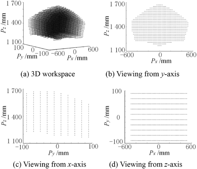

  

  Workspace of 2RPU/UPR PM

• Step 2. Select a set of dimensionless parameters from the optimum region which contains the suitable solutions. As the different coordinates in the optimum region are all eligible, a comparatively better one should be confirmed. So this part of the core work is the comparative analysis of different coordinates.

• Step 3. Determine the normalization factor D by means of the practical work requirements, and then three parameters can be sure.

• Step 4. Check the optimum result. If the obtained parameters conform to the design requirements, the optimizing can stop, or go back to step 2 until the optimizing is successful.

4.4 Results and Validation

With the purpose of better understanding the optimization procedure, an example is given. Here the coordinate (1.4, 0.7) in the optimum region is selected, the three dimensionless parameters are (0.7, 1.438, 0.862). Let a = 200 mm, then $D = \frac{200}{0.7} = 285.714$, so b = r₂·D = 410.857 mm, c = r₃·D = 246.285 mm and the initial distance of point o to the base is 720.41 mm. As the triangles a₁a₂a₃ and A₁A₂A₃ are similar, $e = \frac{bc}{a} = 505.940$ mm.

Considering potential applications, the machine should have a subset workspace in which it can keep an optimum working performance. In order to make the MP be able to move 150 mm along Z-axis, we try to change the distance of the point o to the base. According to the above analysis, we know that the initial distance is 821.465 mm. At this height, the $\text{GTI} = 0.961,$ GOC = 113.770°, and $\text{GFS = } 0. 8 2 5$. For the purpose of enlarging the effective movement, let the distance of point o to the base be 850 mm; then we can get $\text{GTI} = 0.962$, GOC = 114.377° and $\text{GFS = } 0. 8 5 5$. By using the same method, when the distance of the point o to the base is 680 mm, the $\text{GTI} = 0.950$, GOC = 110.206° and $\text{GFS = 0.677}$. After observing and comparing the above data, the effective movement can reach 170 mm. The above results are all satisfy the optimization conditions, so this set of optimization data is available.

Using the above parameters, the structure sketch can be obtained which is shown as Figure 1(a), and this picture is just used to intuitively show the proportional relation of 2RPU/UPR PM after optimal design. By means of the optimized results, the workspace obtained from MATLAB software is shown in Figure 7. Figure 7(a) is the 3-D view, Figure 7(b)‒(c) are the corresponding projected views.

The overall dimensions can be intuitively recognized from the above workspace, which will contribute to analyze the property of this manipulator.

5 Conclusions and Future Work

• (1) A novel 5-DOF HSPM is proposed which is based on the 2RPU/UPR PM. The 2RPU/UPR PM is a new 2R1T PM with two CRAs, so it is easier to implement trajectory planning, parameter calibration, and motion control, compared with the general 2R1T PMs.

• (2) The structure of this machine is described in detail and the kinematics, statics and workspace are all analyzed, which help us to better understanding the structural characteristics and is convenient to optimal design.

• (3) A modified discretization method is used to reveal the workspace of the PM which also could incidentally solve the volume of the workspace.

• (4) The optimal design of 2RPU/UPR PM is presented basing on three indices: GTI, GOC and GFS. The GTI and GOC indices are based on the classical concept of transmission angle, the GFS is a new index which considers the stability of actuated force and is good for improving the mechanical property of actuated system. All of these three indices are independent of any coordinate frame. The optimal results are validated and it is satisfied.

• (5) In our following work, the prototype of the novel 5-DOF HSPM with outstanding performances will be manufactured, and experimental studies will be performed.

References

I Ebrahimi, J A Carretero, R Boudreau. 3-PRRR redundant planar parallel manipulator: Inverse displacement, workspace and singularity analyses. Mechanism and Machine Theory, 2007, 42(8): 1007−1016.
J P Merlet. Parallel robots. Springer Science & Business Media, 2012.
H Xie, S Li, Y F Shen, et al. Structural synthesis for a lower-mobility parallel kinematic machine with swivel hinges. Robotics and Computer-Integrated Manufacturing, 2014, 30(5): 413−420.
Z Huang, Q C Li. Type synthesis of symmetrical lower-mobility parallel mechanisms using the constraint-synthesis method. The International Journal of Robotics Research, 2003, 22(1): 59−79.
S A Joshi, L W Tsai. The kinematics of a class of 3-dof, 4-legged parallel manipulators. Journal of Mechanical Design, 2003, 125(1): 52−60.
P Vischer, R Clavel. Kinematic calibration of the parallel Delta robot. Robotica, 1998, 16(2): 207−218.
J Zhang, Y Q Zhao, J S Dai. Compliance modeling and analysis of a 3-RPS parallel kinematic machine module. Chinese Journal of Mechanical Engineering, 2014, 27(4): 703−713.
Z Huang, Y F Fang. Motion characteristics and rotational axis analysis of 3-Dof parallel robot mechanisms. IEEE International Conference on Systems, Man and Cybernetics, Vancouver, BC, 1995, 1: 67–71.
Y D Xu, D S Zhang, M Wang, et al. Type synthesis of Two-Degrees-of-Freedom rotational parallel mechanism with two continuous rotational axes. Chinese Journal of Mechanical Engineering, 2016, 29(4): 694−702.
K H Hunt. Structural kinematics of in-parallel-actuated robot-arms. Journal of Mechanisms, Transmissions, and Automation in Design, 1983, 105(4): 705−712.
F G Xie, X J Liu, H Zhang, et al. Design and experimental study of the SPKM165, a five-axis serial-parallel kinematic milling machine. Science China Technological Sciences, 2011, 54(5): 1193−1205.
Q C Li, W F Wu, H J Li, et al. A hybrid robot for friction stir welding. Proceedings of the Institution of Mechanical Engineers, Part C: Journal of Mechanical Engineering Science, 2014: 0954406214562848.
Y Y Wang, T Huang, X M Zhao, et al. Finite element analysis and comparison of two hybrid robots-the tricept and the trivariant. IEEE/RSJ International Conference on Intelligent Robots and Systems, Beijing, China, October 9−15, 2006: 490−495.
M Li, T Huang, D G Chetwynd, et al. Forward position analysis of the 3-DOF module of the TriVariant: A 5-DOF reconfigurable hybrid robot. Journal of Mechanical Design, 2006, 128(1): 319−322.
Z M Bi, Y Jin. Kinematic modeling of Exechon parallel kinematic machine. Robotics and Computer-Integrated Manufacturing, 2011, 27(1): 186−193.
Z B Li, Y J Lou, Y S Zhang, et al. Type synthesis, kinematic analysis, and optimal design of a novel class of schönflies-motion parallel manipulators. IEEE Transactions on Automation Science and Engineering, 2013, 10(3): 674−686.
L W Tsai, S Joshi. Kinematics and optimization of a spatial 3-UPU parallel manipulator. Journal of Mechanical Design, 2000, 122(4): 439−446.
X J Liu. Optimal kinematic design of a three translational DOFs parallel manipulator. Robotica, 2006, 24(2): 239−250.
J S Wang, C Wu, X J Liu. Performance evaluation of parallel manipulators: Motion/force transmissibility and its index. Mechanism and Machine Theory, 2010, 45(10): 1462−1476.
F G Xie, X J Liu, T M Li. A comparison study on the orientation capability and parasitic motions of two novel articulated tool heads with parallel kinematics. Advances in Mechanical Engineering, 2013: Article ID 249103.
Y M Song, H Gao, T Sun, et al. Kinematic analysis and optimal design of a novel 1T3R parallel manipulator with an articulated travelling plate. Robotics and Computer-Integrated Manufacturing, 2014, 30(5): 508−516.
J S Wang, X J Liu, C Wu. Optimal design of a new spatial 3-DOF parallel robot with respect to a frame-free index. Science in China Series E: Technological Sciences, 2009, 52(4): 986−999.
D Olaru, G C Puiu, L C Balan, et al. A new model to estimate friction torque in a ball screw system. Product Engineering. Springer Netherlands, 2004: 333−346.
X M Kang, W P Fu, D C Wang, et al. Analysis and testing of axial load effects on ball screw’s friction torque fluctuations. Noise and Vibration Control, 2010, 2: 57−60.
F B Wang, Q H Chen, Q C Li. Optimal design of a 2-UPR-RPU parallel manipulator. Journal of Mechanical Design, 2015, 137(5): 054501.
Z Huang, Y S Zhao, T S Zhao. Advanced spatial mechanism. Beijing: China High Education Publications, 2006.
Y Lu, X L Zhang, C P Sui, et al. Kinematics/statics and workspace analysis of a 3-leg 5-DOF parallel manipulator with a UPU-type composite active constrained leg. Robotica, 2013, 31(2): 183−191.
I A Bonev, J Ryu. A new approach to orientation workspace analysis of 6-DOF parallel manipulators. Mechanism and Machine Theory, 2001, 36(1): 15−28.
A Gallant, R Boudreau, M Gallant. Geometric determination of the dexterous workspace of n-RRRR and n-RRPR manipulators. Mechanism and Machine Theory, 2012, 51: 159−171.
H Ghaffari, G Payeganeh, M Arbabtafti. Kinematic design of a novel 4-DOF parallel mechanism for turbine blade machining. The International Journal of Advanced Manufacturing Technology, 2014, 74(5−8): 729−739.
S Yahya, M Moghavvemi, H Mohamed. Geometrical approach of planar hyper-redundant manipulators: Inverse kinematics, path planning and workspace. Simulation Modelling Practice and Theory, 2011, 19(1): 406−422.
Authors’ Contributions
Y-SZ was in charge of the whole trial; D-SZ wrote the manuscript; D-SZ, Y-DX and J-TY assisted with sampling and laboratory analyses. All authors read and approved the final manuscript.
Authors’ Information
Dong-Sheng Zhang, born in 1988, is currently a PhD candidate at Yanshan University, China. He received his bachelor degree on mechatronics from Yanshan University, China, in 2013. His research interests include parallel manipulator and robotics.
Yun-Dou Xu, born in 1985, is currently an associate professor at School of Mechanical Engineering, Yanshan University, China. He received his bachelor degree and PhD degree from Yanshan University, China, in 2007 and 2012 respectively. His research interests include parallel manipulator and robotics.
Jian-Tao Yao, born in 1980, is currently a professor at School of Mechanical Engineering, Yanshan University, China. He received his bachelor degree and PhD degree from Yanshan University, China, in 2004 and 2010 respectively. His research interests include six-axis force sensors, parallel manipulators, and mechatronics.
Yong-Sheng Zhao, born in 1962, is currently a professor at Yanshan University, China. He received his PhD degree from Yanshan University, China, in 1999. His research interests include mechatronics engineering, robotics and parallel manipulator.
Competing Interests
The authors declare no competing financial interests.
Funding
Supported by National Natural Science Foundation of China (Grant No. 51405425), Key Basic Research Program of Hebei Province’s Applied Basic Research Plan of China (Grant No. 15961805D), and Natural Science Foundation of Hebei Province (Grant No. E2017203387).
Publisher’s Note
Springer Nature remains neutral with regard to jurisdictional claims in published maps and institutional affiliations.
Author information
Authors and Affiliations
Corresponding author
Rights and permissions
Open Access This article is distributed under the terms of the Creative Commons Attribution 4.0 International License (http://creativecommons.org/licenses/by/4.0/), which permits unrestricted use, distribution, and reproduction in any medium, provided you give appropriate credit to the original author(s) and the source, provide a link to the Creative Commons license, and indicate if changes were made.
About this article
Cite this article
Zhang, DS., Xu, YD., Yao, JT. et al. Analysis and Optimization of a Spatial Parallel Mechanism for a New 5-DOF Hybrid Serial-Parallel Manipulator. Chin. J. Mech. Eng. 31, 54 (2018). https://doi.org/10.1186/s10033-018-0251-4
Received:
Accepted:
Published:
DOI: https://doi.org/10.1186/s10033-018-0251-4