Model for the Whole Roller Leveling Process of Plates with Random Curvature Distribution Based on the Curvature Integration Method

Abstract

A model based on the curvature integration method has been applied in an online plate leveling system. However, there are some shortcomings in the current leveling models. On the one hand, the models cannot deal with the leveling process of plates with a random curvature distribution. On the other hand, the current models are suitable only for stable leveling processes and ignore the biting in and tailing out stages. This study presents a new plate-leveling model based on the curvature integration method, which can describe the leveling process of plates with random curvature distribution. Further, the model is solved in two cases in order to take the biting in and tailing out stages into consideration. The proposed model is evaluated by comparing with a plate leveling experiment. Finally, the leveling process of a plate with a wave bent is studied using the proposed model. It is found that the contact angles vary greatly during the biting in and tailing out stages. However, they are relatively steady during the 5 roller leveling stage. In addition, the contact angle of roller No. 2 is the smallest, which is close to 0. Roller leveling can effectively eliminate bending in the plate, but there are regions in the head and tail of the plate, where roller leveling is not effective. The non-leveling region length is about 2 times that of the roller space. This study proposes a quasi-static plate-leveling model, which makes it possible to analyze the dynamic straightening process using a curvature integration method. It also makes it possible to analyze the straightening process of a plate with random curvature distribution.

1 Introduction

A plate is usually subjected to bending deformation during rolling, cooling, transportation, and other processes owing to external forces, temperature changes, and internal forces. Thus, the leveling process is indispensable for flat products. Leveling can effectively eliminate uneven deformation in a plate. Further, residual stress distribution in the plate can also be improved for its further use [1]. The roller leveling process has been widely used in the continuous production of sheet metal thanks to its high efficiency and high effectiveness [2]. In order to meet the increasingly stringent requirements, plate leveling research is focused on developing more accurate leveling models that can fully utilize latest detection and control technology [3].

An effective leveling strategy depends on an accurate analysis of the leveling process, which requires the establishment of a reasonable analytical model. Based on literature survey, analytical models on plate leveling can mainly be divided into three categories. In the first category, leveling analytical models are developed based on the beam bending theory, where the leveling process is studied under an assumption of multi-section and continuous beams [4,5,6,7,8,9,10,11]. This methodology has been widely used to analyze plate and profile leveling processes and some theoretical achievements could be obtained. Zang et al. [12] reported the analytical solution of H-beam bending deflection in the leveling process with nine rollers. Guan et al. [13] studied stress-inheriting behavior during leveling and its influence on the leveling process. Zhou [14] established an analytical model for the roller bending process, where the total deformation curvature is regarded as an independent variable. Liu et al. [15] studied the evolution of stress in a continuous bending process and the effect of the strain hardening model was also studied. Despite being widely available, these models fail to satisfy the ever-increasing requirement for flatness, because the models do not fully consider the contact state between the plate and rollers. The second category consists of finite element method (FEM)-based and boundary element method (BEM)-based analytical models [16,17,18,19,20]. Huh et al. [21] studied the sheet tension leveling process with the help of elastic-plastic finite element simulations. Mathieu et al. [22] simulated a sheet threading process using bridle rolls. Yoon et al. [23] simulated the tension leveling process using 2D and 3D frameworks. It was concluded that 3D simulations should be used for the tension leveling process. The residual stress in a UIC-60 rail after leveling was investigated by Betego´n et al. [24] using 1D, 2D, and 3D simulation models. However, FEM-based analysis of the leveling process is generally time-consuming, which restricts its use in industrial applications. The third category includes the curvature integration method. In this method, a number of iterations are needed to obtain the curvature evolution of the plate in question during the progressive leveling process, in which a relationship between curvature distribution and reduction of rollers is established. Using this method, Kadota et al. [25] studied the leveling process for different materials considering a variable set of process parameters. Instead of the traditional bilinear hardening model, Higo et al. [26] carefully considered the transition behavior of the selected material from an elastic to plastic state and made use of the curvature integration method, consequently improving the prediction of curvature evolution during the leveling process. Xue [27] improved the geometry characterization of the curvature integration method and derived the recurrence formulae of contact angles. Liu et al. [28] studied stress distribution along the width direction. Li et al. [29] studied the effect of an inter-mesh on the residual curvature of a longitudinal profile plate. Thanks to its high accuracy and efficiency, the curvature integration method is preferred for engineering applications. Based on the above analysis, the curvature integration method is selected for the establishment of a target model in this study.

In the current curvature integration models, a plate is usually considered to be bent with a large single curvature during the leveling process. The assumption will inevitably result in an imprecise curvature prediction of the leveled plate. Simultaneously, curvature is generally simplified in the calculation process, where the denominator of the curvature formula is replaced by 1. This simplification causes small errors in solving the curvature. However, an accumulative error is caused when building the relationship between curvature and deflection. Further, the models are effective only for stable leveling stages, because they do not take into consideration the biting in and tailing out stages. The biting in stage will affect the subsequent leveling stage; both ends of the plate are related to the biting in and tailing out stages. Therefore, it is necessary to take biting in and tailing out stages into consideration. Thanks to developments in detection technology, real-time online flatness information of a plate can be obtained. Based on these considerations, this paper presents an online precision leveling model, which is suitable for the current detection technology.

In this study, firstly, the initial deflection curve of a plate is described by a certain function. The curve is discretized into elements of equal length along the longitudinal direction. The accumulated error caused by curvature simplification is discussed in detail. Secondly, a curvature integration model with a high accuracy is established, which can describe the leveling process of a plate with random curvature distribution. To take the biting in and tailing out stages into consideration in addition to the stable leveling stage, the model is solved with contact establishment, and dynamic leveling is considered. Later, the analytical model is experimentally verified. Finally, the proposed model is used to analyze the plate roller leveling process.

2 Curvature Integration Model for the Plate Roller Leveling Process

2.1 Curvature Integration Geometry Model

The initial deflection curve of plate is defined by f(x). Its first derivative g(x) and the second derivative k(x) are as follows:

$$\left\{ {\begin{array}{*{20}c} {g(x) = f^{\prime}(x),} \\ {k(x) = g^{\prime}(x),} \\ \end{array} } \right.$$

(1)

where $x \in [0,L]$ and L is the plate length.

The deflection curve is evenly dispersed into several elements, as shown in Figure 1. The length of the elements along the longitudinal direction is Δx. As the length of the elements is very small, the first derivative and second derivative of the elements on the initial deflection curve can be replaced by the first derivative and second derivative of any point on the elements, respectively. In the current study, the plate end that first enters into the rollers is named as the head and the other end is named as the tail. The elements are numbered from head to tail, as shown in Figure 1. For the element j, Eq. (1) can be rewritten as follows:

Figure 1

Plate deflection curve division

$$\left\{ {\begin{array}{*{20}c} {g(j) = g(j\Delta x),} \\ {k(j) = k(j\Delta x).} \\ \end{array} } \right.$$

(2)

Consequently, the curvature of element j is as follows:

$$A(j) = \frac{{\left| {f^{\prime \prime } } \right|}}{{(1 + {{f^{\prime }}^{2} )^{3/2} }}} = \frac{{\left| {k(j\Delta x)} \right|}}{{(1 + (g(j\Delta x))^{2} )^{3/2} }}.$$

(3)

In the bending process with a small deflection, the denominator of Eq. (3) is generally replaced by 1 in engineering applications, because the item $(g(\Delta xj))^{2}$ is far less than 1. Thus, Eq. (3) can be simplified into the following equation:

$$A(j) = \left| {k(j\Delta x)} \right|.$$

(4)

In the existing curvature integration models, the above simplification is generally adopted in the establishment of a relationship between the curvature and deflection. The basic idea is to establish a geometry model for the first integral and the second integral of the curvature along the plate length direction. However, the above simplification will cause an accumulative error in the deflection curve, which is calculated by curvature distribution. Assuming that there is a curvature error of $\Delta A$in the first element located at the head of the plate during the solving procedure, it will cause a deflection error of $\int_{0}^{L} {\int_{0}^{x} {g\left( 1 \right)\Delta A\text{d}x} \text{d}X}$ at the element of the plate tail, namely, $g\left( 1 \right)\Delta AL^{2} /2$. The error caused by simplification for each element will obviously reduce the solving accuracy of the plate deflection curve, especially in the case of a large curvature deflection. Further, existing models consider the dip angle instead of the slope when building a relationship between slope and deflection, which also causes accumulative error. Therefore, it is necessary to adopt a curvature with less error during the establishment of a curvature integration model.

As the thickness of the plate during leveling remains constant, the deformation in the plate can be described by a plate neutral layer curve. The geometry model of the leveling process is shown in Figure 2.

Figure 2

Plate roller leveling process diagram

Two adjacent rollers together are considered as a leveling span. For leveling with n rollers, the process can be divided into n − 1 leveling spans. The local coordinate system is set up at the contact point between the plate and roller and the corresponding positive direction of the x-axis coincides with the leveling direction of the plate, as shown in Figure 2. The curvature is considered positive when the curve is concave. Correspondingly, the curvature is negative when the curve is convex. In a similar manner, the moment making the plate bend in a concave fashion is defined as positive and the moment responsible for the convex bending of the plate as negative. R is the roller radius. As the plate is replaced by its neutral layer, the roller radius r used in the calculation is the sum of the actual roller radius and half thickness of the plate. L_i is the half length of the roller space, l_i′ is the distance between adjacent contact points along the leveling direction, t_i is the inter-mesh of two adjacent rollers, and t_i′ is the distance between two adjacent contact points along the plate thickness direction. When the contact point of roller i is above the contact point of roller i + 1, t_i and t_i′ are positive. When the contact point of roller i is below the contact point of roller i + 1, t_i and t_i′ are negative. θ_i is the contact angle of roller i with the plate and it is an acute angle. θ_i is positive when it is located in the positive half of the z-axis. Otherwise, θ_i is negative.

When the first roller of leveling span I is the upper roller, the following equation can be established:

$$\left\{ {\begin{array}{*{20}l} {l_{i}^{\prime } = l_{i} - r\theta_{i} - r\theta_{i + 1} ,} \hfill \\ {t^{\prime}_{i} = t_{i} - r\theta_{i}^{2} /2 - r\theta_{i + 1}^{2} /2.} \hfill \\ \end{array} } \right.$$

(5)

When the first roller of leveling span I is the lower roller,

$$\left\{ {\begin{array}{*{20}l} {l_{i}^{\prime } = l_{i} + r\theta_{i} + r\theta_{i + 1} ,} \hfill \\ {t^{\prime}_{i} = t_{i} + r\theta_{i}^{2} /2 + r\theta_{i + 1}^{2} /2.} \hfill \\ \end{array} } \right.$$

(6)

During the leveling process, Eq. (7) can be established for a plate within a leveling span I under the local coordinate system CS_I as follows:

$$\left\{ {\begin{array}{*{20}l} {A_{x} = A_{i} + \Delta A_{x} ,} \hfill \\ {\tan \theta_{x} = \tan \theta_{i} + \int_{0}^{x} {A_{x} (1 + f^{\prime}(x)^{2} )^{3/2} \text{d}x} ,} \hfill \\ {t_{x} = \int_{0}^{x} {\tan \theta_{x} \text{d}x} ,} \hfill \\ \end{array} } \right.$$

(7)

where A_i is the plate reverse bending curvature at the contact point of roller I, A_x is the plate reverse curvature at a distance x from the contact point, ΔA_x is the change in reverse curvature, θ_x is the plate dip angle at a distance x from the contact point, and t_x is the plate deflection at a distance x from the contact point.

When x is equal to l_i′, the location is the contact point between the plate and roller i + 1. As a result, Eq. (7) can be written as:

$$\left\{ {\begin{array}{*{20}l} {\tan \theta_{i + 1} = \tan \theta_{i} + \int_{0}^{{l^{\prime}_{i} }} {A_{x} (1 + f^{\prime}(x)^{2} )^{3/2} {\text{d}}x} ,\;\;\;} \hfill \\ {t^{\prime}_{i} = \int_{0}^{{l^{\prime}_{i} }} {\left( {\tan \theta_{i} + \int_{0}^{x} {A_{x} (1 + f^{\prime}(x)^{2} )^{3/2} {\text{d}}x} } \right){\text{d}}X.} } \hfill \\ \end{array} } \right.$$

(8)

Eq. (8) can be rewritten as

$$\left\{ {\begin{array}{ll} {\tan {\theta _{i + 1}} = \tan {\theta _i} + {A_i}{{\left( {1 + {f^{\prime _i^2}}} \right)}^{3/2}}l_i^\prime }\\ { \qquad \qquad + \int_0^{l_i^\prime } {\Delta {A_x}{{\left( {1 + {f^\prime }{{\left( x \right)}^2}} \right)}^{3/2}}{\rm{d}}x} ,}\\ {{\text{ t}}_i^\prime = \tan {\theta _i}l_i^\prime + {A_i}{{\left( {1 + {f^{\prime _i^2}}} \right)}^{3/2}}{{\left( {{l^\prime }} \right)}^2}/2}\\ { \qquad \qquad + \int_0^{l_i^\prime } {\left( {\int_0^x {\Delta {A_x}{{\left( {1 + {f^\prime }{{\left( x \right)}^2}} \right)}^{3/2}}{\text{d}}x} } \right){\text{d}}X.} } \end{array}} \right.$$

(9)

a_i is defined as the integral value of curvature variation and b_i is the double integral value of curvature variation, as described in:

$$\left\{ {\begin{array}{l} {a_{i} = \int_{0}^{{l^{\prime}_{i} }} {\Delta A_{x} (1 + f^{\prime}(x)^{2} )^{3/2} {\text{d}}x} ,\;\;\;\;\;\;\;\;\;\;} \\ {b_{i} = \int_{0}^{{l^{\prime}_{i} }} {\left( {\int_{0}^{x} {\Delta A_{x} (1 + f^{\prime}(x)^{2} )^{3/2} {\text{d}}x} } \right){\text{d}}X.} } \\ \end{array} } \right.$$

(10)

Thus, Eq. (9) can be rewritten as:

$$\left\{ {\begin{array}{l} {\tan \theta_{i + 1} = \tan \theta_{i} + A_{i} (1 + f^{\prime}_{i} )^{3/2} l^{\prime}_{i} + a_{i} ,\;\;\;} \\ {t^{\prime}_{i} = \tan \theta_{i} l^{\prime}_{i} + A_{i} (1 + f^{\prime}_{i} )^{3/2} \left( {l^{\prime}_{i} } \right)^{2} /2 + b_{i} .} \\ \end{array} } \right.$$

(11)

Eq. (11) can be applied to any leveling span, as the leveling process with n rollers can be divided into n − 1 leveling spans. Thus, a system of equations containing 2(n − 1) equations can be built. If a_i and b_i are given, the independent variables to be identified are the contact angles and reverse curvature of each roller, a total of 2n variables. At the same time, during the plate roller leveling process, the reverse bending curvature A₁ of the first roller is the initial curvature of the plate, which is a known variable. The curvature of the tail roller A_n is the unloading curvature of the reciprocal second roller, which is not an independent variable. Thus, the number of independent unknown variables of equations decreased to 2(n − 1). According to the above analysis, a certain solution exists for the equations (Eq. (11)) of the geometry model. After a_i and b_i are calculated, a full representation of the leveling processes will be established, consequently making a full investigation achievable. Therefore, solving a_i and b_i is the main purpose of the current investigation into the leveling process.

2.2 Solution of the Integral Value of Curvature Variation

In this section, the numerical analytical process of a_i and b_i is described. To take the biting in and tailing out stages into consideration, the solution is constructed under two cases, namely the contact establishment and dynamic leveling phases. It is widely known that plate reverse bending requires at least three rollers. The leveling process starts when the plate head touches the third roller, which is named as the contact establishment phase. After contact establishment, the plate moves forward with the rotation of the rollers; this is named as the dynamic leveling phase. Correspondingly, the next contact is established when the plate head touches the fourth roller. Thus, the leveling process can be regarded as a process of alternating between contact establishment and dynamic leveling.

2.2.1 Contact Establishment Phase

When element 1 touches the nth roller and the element j₁ touches the first roller, the n roller leveling process is established and it can be described by Eq. (12). The subscript 1 in j₁ indicates the number of rollers the element touches and l represents the distance between two rollers:

$$\left\{ {\begin{array}{*{20}l} {n_{1} = l/\Delta x,\;\;\;\;\;\;\;\;} \\ {j_{1} = \left( {n - 1} \right)n_{1} + 1.} \\ \end{array} } \right.$$

(12)

The first roller in the leveling span I is the roller i. When element j_i touches the roller i, the reverse bending curvature of the element j_i can be expressed by $A_{{w(j_{i} )}}$. The initial curvature of element j_i is $A(j_{i} )$, which can be obtained by Eq. (3). The relationship in Eq. (13) is constructed for the total bending curvature $A_{{j_{i} }}$:

$$\left\{ {\begin{array}{*{20}l} {\;j_{i} = j_{1} - (i - 1)n_{1} ,\;\;\;} \\ {A_{{j_{i} }} = A_{{w(j_{i} )}} - A(j_{i} ).} \\ \end{array} } \right.$$

(13)

The bending moment $M_{{j_{i} }}$ of element j_i can be obtained from its total bending curvature $A_{{j_{i} }}$, as discussed in Ref. [30]. In the same manner, the total bending curvature $A_{{j_{i + 1} }}$ and bending moment $M_{{j_{i + 1} }}$ of element j_i + 1 that touches the roller i + 1 can be obtained.

In the leveling span I, the bending moment distribution of the plate between two adjacent rollers is linear. As long as $M_{{j_{i} }}$ and $M_{{j_{i + 1} }}$ are obtained, the bending moment of an arbitrary element j between roller i and roller i + 1 can be calculated using the following equation:

$$M_{j} = M_{{j_{i} }} + \frac{{M_{{j_{i + 1} }} - M_{{j_{i} }} }}{{n_{1} }}(j - j_{i} ).$$

(14)

The total bending curvature $A_{j}$ of the element j within the leveling span I can be obtained from its bending moment M_j, which can be described as follows:

(1) Assuming that the material behaves as an ideal elastic-plastic, the relationship between the curvature and moment of the simple bending process follows Eq. (15), as discussed in Ref. [6]. In the equation, M_t is the maximum bending moment of flexible bending and A_t is the maximum bending curvature of flexible bending. The inverse function of Eq. (15) can be expressed as Eq. (16). The subscript of $A_{j}^{0}$ represents the number of the calculated element and the superscript represents the number of iterations, as the solving process needs iteration. When the superscript is 0, the variable is the initial value. The item ${\text{sgn}}(M_{j} )$ is to preserve the sign of M_j.

$$M_{j} = M_{t} \left( {1.5 - 0.5\frac{{A_{t}^{2} }}{{(A_{j}^{0} )^{2} }}} \right),$$

(15)

$$A_{j}^{0} = {\text{sgn}}(M_{j} )A_{t} \sqrt {\left( {3 - 2\frac{{M_{j} }}{{M_{t} }}} \right)^{ - 1} } .$$

(16)

(2) The bending moment $M_{j}^{0}$ can be calculated according to $A_{j}^{0}$. If $\left| {M_{j}^{0} } \right| > \left| {M_{j} } \right|$, the total bending moment A_j is between 0 and $A_{j}^{0}$. When the upper and lower bounds of the total curvature are determined, the numerical solution of the total bending curvature in the given error range can be obtained using a dichotomous method. If $\left| {M_{j}^{0} } \right| < \left| {M_{j} } \right|$, $A_{j}^{1}$ is considered as $2A_{wj}^{0}$. Subsequently, the moment $M_{j}^{1}$ is calculated according to $A_{j}^{1}$. If $\left| {M_{j}^{1} } \right| > \left| {M_{j} } \right|$, it indicates that the total bending moment A_j is between $A_{j}^{0}$ and $A_{j}^{1}$. The dichotomy method is used to find the numerical solution of A_j. If $\left| {M_{j}^{1} } \right| < \left| {M_{j} } \right|$, $A_{j}^{2}$ is considered as $3A_{j}^{0}$. In this case, the numerical solution for the total bending curvature within a given error range can be obtained.

When the total bending curvature $A_{j}$ of element j is obtained, its initial curvature is $A(j)$, which is calculated by Eq. (3). Its reverse bending curvature follows as

$$A_{wj} = A_{j} - A(j).$$

(17)

As the curvature of the element is obtained, the solving steps of its slope are as follows.

(1) Because the moment of element $j_{1}$ that touches the first roller is 0, its slope does not change during leveling. Its slope $g_{{j_{1} }}$ can be solved according to Eq. (2). $g_{{j_{1} - 1}}^{0}$, which is the initial slope of element $(j_{1} - 1)$, is initially set as $g_{{j_{1} }}$. $g_{{j_{1} - 1}}^{1}$ can be calculated from Eq. (18). If the relative change in the two values is less than the given precision, the iteration stops. If the relative change in the two values is greater than the given precision, $g_{{j_{1} - 1}}^{2}$ is calculated according to $g_{{j_{1} - 1}}^{1}$. The iteration is run until the relative error of $g_{{j_{1} - 1}}^{m - 1}$ and $g_{{j_{1} - 1}}^{m}$ is less than the given precision:

$$\left\{ {\begin{array}{l} {g_{{j_{1} - 1}}^{m} = g_{{j_{1} - 1}}^{m - 1} + A_{{wj(j_{1} - 1)}} (1 + (g_{{j_{1} - 1}}^{m - 1} )^{2} )^{3/2} \Delta x,\;} \\ {\vartheta = \left| {(g_{{j_{1} - 1}}^{m} - g_{{j_{1} - 1}}^{m - 1} )/g_{{j_{1} - 1}}^{m - 1} } \right|.\;\;\;\;\;\;\;\;\;\;\;\;\;\;\;\;\;\;\;} \\ \end{array} } \right.$$

(18)

(2) After the slope $g_{j}$ of element j is obtained, $g_{j}$ is used as the initial value of element j − 1. The slope of element j − 1 can be calculated according to the above step. The calculation keeps running until the slopes of all the elements are evaluated.

After calculating the slopes and reverse curvatures of all the elements, the first integral value of curvature variation a_i and second integral value of curvature variation b_i of the leveling interval I are:

$$\left\{ {\begin{array}{*{20}l} {a_{i} = \sum\limits_{k = 1}^{{n_{2} }} {[A_{{j_{i} - k}} (1 - g_{{j_{i} - k}}^{2} )^{3/2} - A_{{j_{i} }} (1 - g_{{j_{i} }}^{2} )^{3/2} ]\Delta x,\;\;\;\;\;\;\;\;\;\;\;\;\;\;} } \\ {b_{i} = \sum\limits_{p = 1}^{{n_{2} }} {\left\{ \begin{array}{l} \sum\limits_{k = 1}^{p} {[A_{{j_{i} - k}} (1 - g_{{j_{i} - k}}^{2} )^{3/2} - A_{{j_{i} }} (1 - g_{{j_{i} }}^{2} )^{3/2} ]} \hfill \\ + \sum\limits_{k = 1}^{p + 1} {[A_{{j_{i} - k}} (1 - g_{{j_{i} - k}}^{2} )^{3/2} - A_{{j_{i} }} (1 - g_{{j_{i} }}^{2} )^{3/2} ]} \hfill \\ \end{array} \right\}\Delta x^{2} } /2.} \\ \end{array} } \right.$$

(19)

The initial reverse bending curvatures and contact angles of leveling rollers are given. The calculated results are used as inputs for iteration, until the relative error of the calculated bending curvatures and input curvatures is less than the given precision. The numerical analysis process of the leveling establishment phase is shown in Figure 3.

Figure 3

Curvature integration model analysis flow chart in the contact establishment phase

2.2.2 Dynamic Leveling Phase

After contact is established, the plate moves forward as the leveling rollers rotate. The dynamic leveling process is analyzed according to the length of the plate moving forward. As the plate is discretized into elements whose length is Δx, the analysis step increment is uΔx, where u is a positive integer. The curvature and stress distribution in the previous step will inevitably impact the subsequent leveling process; the curvature and section stress of the elements obtained from the previous step are regarded as the initial state for subsequent computations. The above-mentioned contact establishment phase is taken as the initial state of the dynamic leveling phase. When the plate advances by uΔx, the numbers of elements whose curvature and section stress change are 1~j₁ + u. These elements can be classified into three categories. The solutions corresponding to their curvatures are as follows.

The first group consists of elements that move away from the leveling span. The reverse bending effect of the previous analysis step vanishes. Elements 1 − u are analyzed in this step.

In the preceding analysis step, the bending moment and reverse bending curvature of element j are M_j and A_wj respectively, which are known quantities. Curvature after rebounding $(A_{j} )_{2}$ in the current analysis step can be calculated from M_j and A_wj. The subscript 2 of $(A_{j} )_{2}$ means that the variable represents the current state of the plate and it helps to distinguish from the state of the previous analysis step.

The second group consists of elements entering the leveling span. These elements do not enter the leveling roller originally. During the forward movement of the plate, they enter the leveling span and are bent. These elements numbers are j₁ + 1 to j₁ + u and they are located in the first leveling span.

At this time, the 2nd roller comes into contact with the element whose number is j₁ + u − n₁. $(A_{{w(j_{1} + u - n_{1} )}} )_{2}$ is assigned as the reverse bending curvature of the element j₁ + u − n₁. Its initial curvature $(A_{{\left( {j_{1} + u - n_{1} } \right)}} )_{2}$ in the current analysis step is the reverse bending curvature $A_{{w\left( {j_{1} + u - n_{1} } \right)}}$ of the previous analysis step. In this way, the total bending curvature $(A_{{(j_{1} + u - n_{1} )}} )_{2}$ can be calculated using Eq. (13). Later, the bending moment $(M_{{n_{1} + u + 1}} )_{2}$ can be solved from its total bending curvature $(A_{{(j_{1} + u - n_{1} )}} )_{2}$. As the bending moment of the first roller is zero, the bending moment of the elements j₁ + 1 to j₁ + u can be solved using Eq. (14). When the moments of these elements are known, their reverse bending curvatures can be obtained.

The third group consists of elements whose bending moments change with the movement of the plate. These elements are numbered u + 1 to j₁.

Firstly, the bending moments of the elements that touch each roller are calculated. Later, the bending moments of the elements u + 1 to j₁ are calculated using Eq. (14). For element j, whose number is in between u + 1 and j₁, the absolute value of the bending moment (M_j)₂ is subtracted from the absolute value of the bending moment M_j of previous analysis step, as shown in Eq. (20). If M_j′ is greater than 0, it indicates that the element j is in the loading process. If M_j′ is less than 0, it indicates that the element j is in the unloading process:

$$M_{j}^{\prime } = \left| {(M_{j} )_{2} } \right| - \left| {M_{j} } \right|.$$

(20)

Assuming that the element j is in the loading process, the increment in bending moment, which is represented by ΔM_j, can be calculated as shown in Eq. (21):

$$\Delta M_{j} = (M_{j} )_{2} - M_{j} .$$

(21)

In this case, the increase in the reverse bending curvature of the element needs to be solved; the corresponding numerical analysis steps are as follows:

(1) Assuming that the material satisfies the ideal elastic-plastic model, a derivative function of Eq. (16) is derived and the curvature increment can be obtained as the initial value, as shown in Eq. (22):

$$\Delta A_{j}^{0} = A_{t} \sqrt {\left( {3 - 2\frac{{M_{j} }}{{M_{t} }}} \right)^{ - 3} } \Delta M_{j} .$$

(22)

(2) Because the section stress of element j in the previous step is σ_wj, the new section stress $\sigma_{wj}^{0}$ caused by curvature increment $\Delta A_{j}^{0}$ can be calculated. Later, the element moment $(M_{j} )_{2}^{0}$ is calculated using $\sigma_{wj}^{0}$. If $\left| {(M_{j} )_{2}^{0} - M_{j} } \right| > \left| {\Delta M_{j} } \right|$, it indicates that the curvature increment is between 0 and $\Delta A_{j}^{0}$. The numerical solution of total bending curvature in the given error range can be obtained using a dichotomous method. If $\left| {(M_{j} )_{2}^{0} - M_{j} } \right| < \left| {\Delta M_{j} } \right|$, $\Delta A_{j}^{1}$ is considered as $2\Delta A_{j}^{0}$. Subsequently, the bending moment $(M_{j} )_{2}^{1}$ is calculated from $\Delta A_{j}^{1}$. If $\left| {(M_{j} )_{2}^{1} - M_{j} } \right| > \left| {\Delta M_{j} } \right|$, it indicates that the curvature increment is between $\Delta A_{j}^{0}$ and $\Delta A_{j}^{1}$, and the total bending curvature is obtained using a dichotomous method. If $\left| {(M_{j} )_{2}^{1} - M_{j} } \right| < \left| {\Delta M_{j} } \right|$, $\Delta A_{j}^{2}$ is considered as $3\Delta A_{j}^{0}$. In this case, the numerical solution for the increment in the reverse bending curvature within a given error range can be obtained.

When the element curvature increment $\Delta A_{j}$ is obtained, its reverse bending curvature satisfies the following equation:

$$(A_{wj} )_{2} = A_{wj} + \Delta A_{j} .$$

(23)

For elements in the unloading process, the solution procedures corresponding to the curvature increments are roughly the same as those for the elements in the loading process. The difference lies in the solution of section stress. The section stress for loading elements is given by the superposition of the bending stress and previous section stress. However, the section stress for unloading elements is given by the superposition of the rebounding stress and previous section stress.

The numerical analysis process corresponding to the dynamic leveling phase is shown in Figure 4.

Figure 4

Curvature integration model analysis flow chart in the dynamic leveling phase

3 Verification

In order to evaluate the performance of the proposed model, an experimental study of the plate roller leveling process was conducted. The results obtained from the curvature integration model are compared with the experimental results.

3.1 An Experimental Plate and Leveling Machine

A cold-rolled 409L stainless steel plate was selected as the experimental material. Tensile tests were conducted to obtain the material mechanical parameters. The geometrical parameters of the specimen are shown in Figure 5 and the test results are shown in Figure 6. As the reinforcement effect of the material is weak, the material is considered an ideal elastic-plastic material. The Young’s modulus was found to be 210 GPa, while the yield limit was 245 MPa.

Figure 5

A tensile test specimen

Figure 6

Experimental plate parameters

The experimental leveling machine is shown in Figure 7(a). The width of the leveling roller was 500 mm; the leveling speed varied from 0.1 m/s to 10 m/s and the motor power was 5 kW. To ensure a stable leveling length, only 5 rollers were used during leveling, as the length of the plate was 1000 mm. The arrangement of the 5 rollers is illustrated in Figure 7(b).

Figure 7

Experimental leveling machine: (a) Leveling machine; (b) Roller arrangement

3.2 Plate Shape Measurement

The deflection curve of the leveled plate can be used as a key index to evaluate the leveling process. Meanwhile, curvature distribution can be calculated from the plate deflection curve. Therefore, the deflection curve is measured using a 3D laser scanner. It should be mentioned that the plate thickness is nearly constant during the process. Thus, surface topography obtained from the 3D laser scanner is used to describe plate deformation during leveling. The measurement process is detailed as follows.

• (1) Positioning marker arrangement. The positioning markers are glued to the plate surface to be measured, as shown in Figure 8(a). The markers are coated with a special reflective material. They reflect the light emitted by the device and the reflected data is received by same device.

  Figure 8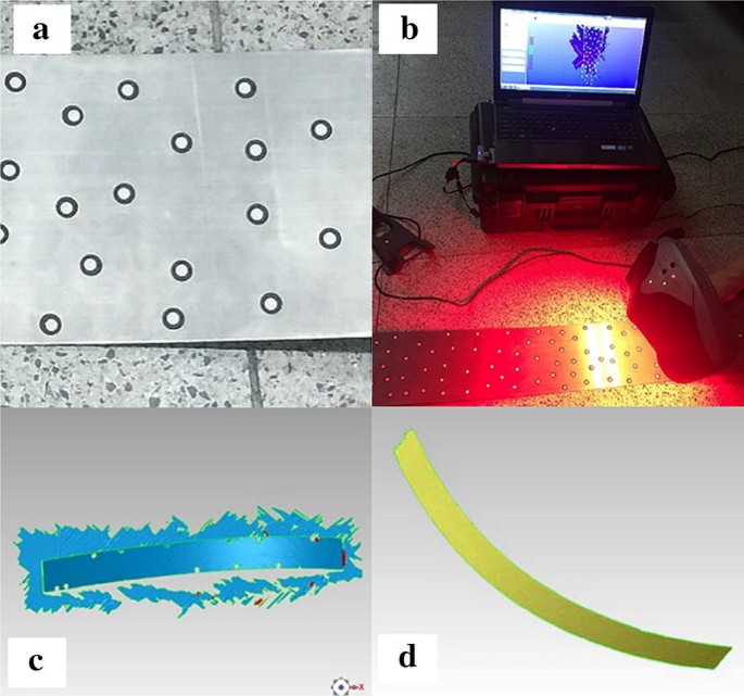

  

  Measurement process: (a) Positioning marker arrangement; (b) Data acquisition site; (c) Model post-processing; (d) Surface topography model

• (2) Data acquisition of the plate surface topography. The plate surface is scanned with a laser scanner. The data is transmitted to the computer and a data acquisition software is used for real-time modeling, as shown in Figure 8(b).

• (3) Surface model post-processing. The model is imported into the post-processing software Geomagic Studio^TM. The holes in the plate model are repaired during the scanning process and the excess parts are removed, as shown in Figure 8(c).

• (4) Surface topography model. The post-processing surface topography model is shown in Figure 8(d). The model can be imported into 3D physical modeling software, such as Solidworks^TM and ProE^TM to obtain further information, such as surface curvature and deflection.

3.3 Results and Discussion

Leveling experiments were conducted to evaluate the proposed model. The inter-mesh of roller 2 was 1.5 mm, while that of roller 4 was 0.8 mm. The plate before and after leveling is shown in Figure 9. The surface scanning results are shown in Figure 10. The deflection curve before leveling is extracted along the middle of the plate and fitted with the function shown in Eq. (24):

Figure 9

Experimental plate: (a) Before leveling; (b) After leveling

Figure 10

Surface scanning results: (a) Before leveling; (b) After leveling

$$z = ax^{4} + bx^{3} + cx^{2} + dx + e,$$

(24)

where a = − 4.898 × 10⁻⁹, b = − 8.28 × 10⁻⁶, c = − 5.11 × 10⁻³, d = 1.844, and e = 21.16.

Deflection curves along the length direction of the plate obtained experimentally and by model parsing are shown in Figure 11. The maximum error of the deflection curve between experimental and model analyses is 2.6 mm. Because the model calculation results are very close to the experimental results, it can be concluded that the proposed model can predict the plate leveling process effectively.

Figure 11

Plate deflection curve

4 Simulation Results and Discussion

The proposed model was verified in Section 3. In this section, the model is used to predict the plate leveling process. Taking the plate roller leveling process mentioned above as the research object, the leveling parameters are shown in Table 1. The initial deflection curve function of the plate in question is shown in Eq. (25):

Table 1 Leveling parameters

$$z = 30\sin \frac{{\uppi{x}}}{500}.$$

(25)

Δx is set as 0.5 mm and u is 10. The plate goes through 200 analysis steps during the leveling process, which can be divided into 3 stages, namely the biting in stage, the 5 roller leveling stage, and the tailing out stage.

As mentioned earlier, the contact angle has a remarkable impact on plate curvature. Therefore, it is necessary to discuss contact angle values during the leveling process. The plate contact angles of each roller are calculated using the proposed model, as shown in Figure 12. It can be seen that the contact angles vary greatly during the biting in stage and tailing out stage; they are relatively constant except for roller No. 1 during the 5 roller leveling stage. In addition, the contact angle of roller No. 2 is the smallest, which is close to 0.

Figure 12

Contact angle analysis

Curvature is also a key parameter to study the leveling process and evaluate the leveled plate. Curvature distribution before leveling and after leveling is shown in Figure 13. It can be seen that plate bending is eliminated significantly after the roller leveling process. However, for the head and tail regions of the plate, roller leveling is not effective. That is to say that there are regions at the plate head and end that cannot be leveled by the roller leveling method. The non-leveling region length is nearly 200 mm, about 2 times greater than the roller space.

Figure 13

Curvature distribution

The plate deflection curve directly reflects the leveling effect. The plate deflection curves before and after leveling are shown in Figure 14. It can be seen from the figure that plate deflection obviously decreased after the leveling process. As the bending curvatures of the head region and tail region are hard to eliminate, the plate shape curve includes warping in these regions.

Figure 14

Plate deflection curve

$\int_{ - H/2}^{H/2} {\left| {\sigma_{z} } \right|{\text{d}}z} /H\sigma_{s}$ is defined as the absolute stress ratio and $\left| {\sigma_{H/2} } \right|/\sigma_{s}$ is defined as the surface stress ratio. The absolute stress ratio and surface stress ratio of the leveled plate are shown in Figure 15. According to the stress distribution, the plate can be divided into 4 regions. Region 1 is the plate head region, region 2 is the plate middle region, which is close to the head, region 3 is the plate middle region close to the tail, and region 4 is the plate tail region. It can be seen from the figure that the residual stress is initially zero and then rapidly increased in region 1 and region 4 of the plate. The maximum value of residual stress is found in region 1. The theoretical demarcation point of the surface residual stress distribution of region 2 and region 3 is 500 in the length direction. However, the actual demarcation point is less than 500 because of advanced contact, which is responsible for the contact angle. Distribution of the surface residual stress in region 2 and region 3 is basically symmetrical, but the absolute stress in region 2 is far greater than that in region 3.

Figure 15

Residual stress

5 Conclusions

• (1) The curvature of the plate should be solved precisely and the slope should be calculated to avoid errors in deflection calculation. To take the biting in and tailing out stages into consideration, the proposed curvature integration model is solved in two phases, which include the contact establishment phase and dynamic leveling phase.

• (2) A plate leveling experiment was conducted. The proposed model was verified by comparing the deflection curves obtained from the proposed model and experiments.

• (3) The contact angle varies greatly during the biting in and tailing out stages, but it is mostly relatively constant during the stable leveling stage. The roller leveling process has a significant effect on eliminating plate bending, but it can hardly work in the head and tail regions of the plate.

References

W Grimm, J Korth, W Kohler. Ilsenburg heavy-plate mill: Modernisation of the mill stand area and of the hot-plate leveler. Iron Steel Review, 2008, 51(9): 11.
V Philippaus, S Mailllard. Modern levelers for advanced plate grade. Iron Steel Review, 2009, 52(10): 144.
H Z Xu, K Liu, X H Peng, et al. Research of the image processing in dynamic flatness detection based on improved laser triangular method. Academic Journal of Xi’an Jiaotong University, 2008, 20(3): 168–171.
F Cui. Straightening and straightening machine. 2nd ed. Beijing: Metallurgy Industry Press, 2002. (in Chinese)
A R He, D Z Liu, C Liu. Research on roller straightening mechanical behavior of plastic hardening material. Journal of Mechanical Engineering, 2016, 52(18): 85–91. (in Chinese)
Z Y Ma, L F Ma, R J Wang, et al. Study on control strategies of two-roll straightening for bar high precision straightening. Journal of Mechanical Engineering, 2017, 53(20): 77–88. (in Chinese)
Q H Fan, H Zhang, X C Jiang. Leveling theory and experiment study on high strength steel plate of excavator working arm. Journal of Mechanical Engineering, 2017, 53(8): 82–90. (in Chinese)
G C Yu, J Zhao, R Ma, et al. Uniform curvature theorem by reciprocating bending and its experimental verification. Journal of Mechanical Engineering, 2016, 52(18): 57–63. (in Chinese)
J Zhao, H Q Cao, P P Zhan, et al. Pure bending equivalent principle for over-bend straightening and its experimental verification. Journal of Mechanical Engineering, 2012, 48(8): 28–33. (in Chinese)
Z Q Zhang, Y H Yan, H L Yang. Research of section deformation of brazier effect in continuous straightening a thin-walled tube. Journal of Mechanical Engineering, 2015, 51(10): 62–68. (in Chinese)
Z Q Zhang, Y H Yan, H L Yang. The straightening curvature-radius model for the thin-walled tube and its validation. Journal of Mechanical Engineering, 2013, 49(21): 160–167. (in Chinese)
Y Zang, H G Wang, F L Cui. Elastic-plasticity analyze of bending deflection on section roller straightening. Journal of Mechanical Engineering, 2005, 41(11): 47–52. (in Chinese)
B Guan, Y Zang, X N Pang, et al. Stress distribution and reverse bending behavior of section during roller leveling process. Journal of Central South University (Science and Technology), 2012, 43(5): 1740–1745.
C L Zhou. Simulation and mathematical model on hot plate roller leveling. Shenyang: Northeastern University, 2006. (in Chinese)
D Y Liu, A R He, H B Wang, et al. Reverse bending research of leveling on plastic hardening material. Journal of Mechanical Engineering, 2015, 51(8): 76–82. (in Chinese)
M Grüber, G Hirt. A strategy for the controlled setting of flatness and residual stress distribution in sheet metals via roller levelling. Procedia Engineering, 2017, 207: 1332–1337.
M Laugwitz, S Seuren, M Jochum, et al. Development of levelling strategies for heavy plates via controlled FE models. Procedia Engineering, 2017, 207: 1349–1354.
H L Gui, Q Li, Q X Huang. The influence of bauschinger effect in straightening process. Mathematical Problems in Engineering, 2015(4): 1–5.
H L Gui, Q Li, Y Li, P Li, Q X Huang. Analysis of rolled piece deformation in straightening process using Fm-Bem. Journal of Marine Science and Technology-Taiwan, 2014(22): 550–556.
Q D Zhang, S Zhou, X F Zhang, et al. Analytic modeling and corroborating by FEM of tension leveling process of thin buckled steel strip. Journal of Mechanical Engineering, 2015, 51(2): 49–57. (in Chinese)
H Huh, H W Lee, R P Sang, et al. The parametric process design of tension levelling with an elasto-plastic finite element method. Journal of Materials Processing Technology, 2001, 113(1): 714–719.
N Mathieu, R Dimitriou, A Parrico, et al. Flatness defects after bridle rolls: a numerical analysis of leveling. International Journal of Material Forming, 2013, 6(2): 255–266.
J Yoon. Numerical simulation of continuous tension leveling process of thin strip steel and its application. Journal of Iron and Steel Research, 2007, 14(6): 8–13.
C Betego´n Biempica, J J del Coz Dı´az, P J Garcia Nieto, et al. Nonlinear analysis of residual stresses in a rail manufacturing process by FEM. Applied Mathematical Modelling, 2009, 33: 34–53.
K Kadota, R Maeda. A model of analysis of curvature in leveling process-numeric study of roller leveling process. Jpn. Soc. Technol. Plast., 1993, 34: 481–486.
T Higo, H Matsumoto, S Ogawa. Effects of numerical expression of stress-stain curve on curvature of material of roller leveling process. Jpn. Soc. Technol. Plast., 2002, 43(496): 439–443.
J A Xue. Theoretical analysis for plate leveling process and its control system. Shenyang: Northeastern University, 2009. (in Chinese)
Z F Liu, Y Q Wang, X C Yan. A new model for the plate leveling process based on curvature integration method. International Journal of Mechanical Sciences, 2012, 54: 213–224.
L Cui, Q Q Shi, X H Liu, et al. Residual curvature of longitudinal profile plate roller in leveling process. Journal of Iron and Steel Research, 2013, 20(10): 23–27.
B Guan, Y Zang, D P Wu, et al. Stress-inheriting behavior of H-beam during roller straightening process. Journal of Materials Processing Technology, 2017, 244: 253–272.
Authors’ Contributions
BG, YZ and CZ conceived the model framework; CZ and BG was in charge of the whole trial; CZ and BG wrote the manuscript; YW assisted with sampling and laboratory analyses. All authors read and approved the final manuscript.
Authors’ Information
Ben Guan, born in 1985, is currently an associate professor at School of Mechanical Engineering, University of Science and Technology Beijing, China. He is also a research associate at Institute of Artificial Intelligence, University of Science and Technology Beijing, China.
Chao Zhang, born in 1990, is currently a PhD. He received his philosophy degree from University of Science and Technology Beijing, China.
Yong Zang, born in 1963, is currently a Prof. at School of Mechanical Engineering, University of Science and Technology Beijing, China.
Yuan Wang, born in 1989, is currently a PhD candidate at School of Mechanical Engineering, University of Science and Technology Beijing, China.
Competing Interests
The authors declare that they have no competing interests.
Funding
Supported by National Hi-tech Research and Development Program of China (863 Program, Grant No. 2013AA031302), and National Natural Science Foundation of China (Grant No. 51805024).
Author information
Authors and Affiliations
Corresponding author
Rights and permissions
Open Access This article is distributed under the terms of the Creative Commons Attribution 4.0 International License (http://creativecommons.org/licenses/by/4.0/), which permits unrestricted use, distribution, and reproduction in any medium, provided you give appropriate credit to the original author(s) and the source, provide a link to the Creative Commons license, and indicate if changes were made.
About this article
Cite this article
Guan, B., Zhang, C., Zang, Y. et al. Model for the Whole Roller Leveling Process of Plates with Random Curvature Distribution Based on the Curvature Integration Method. Chin. J. Mech. Eng. 32, 47 (2019). https://doi.org/10.1186/s10033-019-0361-7
Received:
Accepted:
Published:
DOI: https://doi.org/10.1186/s10033-019-0361-7