On Generating Expected Kinetostatic Nonlinear Stiffness Characteristics by the Kinematic Limb-Singularity of a Crank-Slider Linkage with Springs

Abstract

Being different from avoidance of singularity of closed-loop linkages, this paper employs the kinematic singularity to construct compliant mechanisms with expected nonlinear stiffness characteristics to enrich the methods of compliant mechanisms synthesis. The theory for generating kinetostatic nonlinear stiffness characteristic by the kinematic limb-singularity of a crank-slider linkage is developed. Based on the principle of virtual work, the kinetostatic model of the crank-linkage with springs is established. The influences of spring stiffness on the toque-position angle relation are analyzed. It indicates that corresponding spring stiffness may generate one of four types of nonlinear stiffness characteristics including the bi-stable, local negative-stiffness, zero-stiffness or positive-stiffness when the mechanism works around the kinematic limb-singularity position. Thus the compliant mechanism with an expected stiffness characteristic can be constructed by employing the pseudo rigid-body model of the mechanism whose joints or links are replaced by corresponding flexures. Finally, a tri-symmetrical constant-torque compliant mechanism is fabricated, where the curve of torque-position angle is obtained by an experimental testing. The measurement indicates that the compliant mechanism can generate a nearly constant-torque zone.

1 Introduction

A mechanism with springs is defined as a rigid-body linkage whose joints are placed springs. For this type of mechanisms, the kinetostatic driving force/torque of this type of mechanisms is nonlinear with respect to the position parameter. The nonlinear relation between the driving force/torque and the position parameter is called kinetostatic nonlinear stiffness characteristic. The mechanism with springs possessing this characteristic can be applied in constant force mechanism [1], vibration isolator [2] and gravity balancer [3]. The mechanism attached springs is often used in the type synthesis of compliant mechanisms based on the rigid-body replacement method and the compliant mechanisms analysis based on the pseudo-rigid-body model [4,5,6]. Compliant mechanisms can be fabricated in monolithic and are applied in many applications needing high precision because of absence of backlash and friction [7], such as energy harvester based on buckled beam [8, 9], micro-switch [10] and high accurate driver [11]. However, the buckled beam only generates bi-stability but other nonlinear stiffness characteristics. Moreover, the mechanical model of bi-stable buckled beam is very complicated [12, 13]. The four-bar linkage with placed springs can be used to design compliant mechanisms with bi-stable behavior by employing pseudo-rigid-body replacement [14], which develops the configuration of the bi-stable mechanism.

When the rigid-body replacement method is use to synthesize compliant mechanisms processing corresponding performance, designers should grasp series of performances of the rigid-body linkage. Thus one should have much experience on linkage design and performance analysis. Therefore, it is meaningful that some common attributes are used to construct compliant mechanisms with nonlinear stiffness characteristic.

Kinematic singularity which is a basic property of linkages affects the performance of linkages seriously, so many scholars pay much attention on singularity distribution, singularity property identification and singularity avoidance [15, 16]. However, kinematic singularity has two sides, and can be used to construct new types of devices. Kinematic singularity of the spatial parallel linkage whose links are connected by universal joints are used to construct several types of reconfigurable parallel mechanisms [17]. When parallel mechanisms work near the singularity, they are sensitive to external load. This property is applied to design the force sensors [18, 19]. A new compliant mechanism with negative-stiffness characteristic is synthesized by using kinematic singularity of a four-bar linkage [20]. The planar parallelogram linkage when the two cranks are collinear is used to construct a type of reconfigurable compliant gripper by applying rigid-body replacement method [21]. A new medical device is designed by using the property that a parallel mechanism obtains an additional freedom when it is singular [22].

In this paper, by the crank-slider mechanism with springs as an example, the kinematic limb-singularity which is a common property of rigid-body linkages, is used to construct the kinetostatic nonlinear stiffness characteristic. The rest of the paper is organized as follows: Section 2 addresses the kinetostatic model of the mechanism and Section 3 classifies nonlinear stiffness characteristics as four types. Section 4 analyzes the influences of spring stiffness on the nonlinear stiffness characteristics generated by the mechanism when moves from nonsingular position and passes the kinematic limb-singularity position. Section 5 indicates that the mechanism only produces positive-stiffness characteristic when moves from the kinematic limb-singularity position to nonsingular position. Section 6 describes the approach by creating an expected zero-stiffness (constant-torque) characteristic of the mechanism working around the kinematic limb-singularity position. In Section 7, design of a nonlinear compliant mechanism is further discussed and is validated by the experimental testing. Finally, Section 8 draws some important conclusions.

2 Kinetostatic Model of the Mechanism

Figure 1 shows the schematic of the crank-slider mechanism with springs. Crank AB rotates about pin joint A in anticlockwise and drives the slider to moves along the horizontal line, where link AB and slider are connected by coupler BC. Three pin joints are placed torsional springs whose stiffness is K_RA, K_RB and K_RC, respectively. Prismatic joint C is added extension spring whose stiffness is K_PC.

Figure 1

Crank-slider linkage with springs

The Cartesian coordinates system, O-xyz, is attached on the base, where origin O is fixed on point A, the positive direction of x-axis points to the horizontal right, the positive direction of y-axis is vertically up, and z-axis is determined by the right-hand rule.

Vectors AB and BC are defined by r₁ and r₂, respectively. Projects of vector position C on the x-axis and y-axis with respect to the frame O-xyz are defined by r₃ and e, respectively. Scalars r₁ and r₂ are lengths of links AB and BC, respectively. Scalars r₃ and e are the coordinates of point C on the x-axis and y-axis, respectively. Link-length, r₁ and r₂, and offset, e, should satisfy

$$- \left( {r_{ 1} + r_{ 2} } \right) < e < r_{ 1} + r_{ 2},$$

(1)

so as to allow the mechanism to pass through the right limiting position, which is called the kinematic limb-singularity and occurs when the crank and coupler are along the same line.

Here we suppose that there is no friction and clearance between any two links connected by a kinematic pair. Moreover, we only discuss the kinetostatic model of the mechanism during the motion rather than considering any inertial force/torque and gravity caused by links quality.

The driving torque applied on link AB is set as

$$\varvec{T}_{\text{d}} = T_{\text{d}} \varvec{k},$$

(2)

where vector k is the unit vector of z-axis (vectors i and j are unit vectors of x-axis and y-axis, respectively). Torque vector T_d is along the z-axis, scalar ||T_d|| is the magnitude of driving torque T_d, where T_d > 0 indicates T_d is along the positive direction of z-axis and T_d < 0 corresponds to direction of T_d pointing to negative z-axis.

The angular displacement of pin joint A is

$$\varvec{\varPsi}_{\text{A}} = \left( {\theta_{\text{A}} - \theta_{{{\text{A}}0}} } \right)\varvec{k},$$

where θ_A is the rotation angle of x-axis to link AB and indicates the input position angle of link AB, θ_A0 corresponds to the initial angle. In this paper, value of θ_A allows no spring lose efficacy.

Here we consider θ_A as the general coordinate of the mechanism. Thus the virtual angular displacement of joint A is

$$\updelta\varvec{\varPsi}_{\text{A}} = \frac{{{\text{d}}\varvec{\varPsi}_{\text{A}} }}{{{\text{d}}\theta_{\text{A}} }}\updelta\theta_{\text{A}} =\updelta\theta_{\text{A}} \varvec{k}.$$

The virtual work caused by driving torque, T_d, is

$${\updelta}{W}_{\text{d}} = \varvec{T}_{\text{d}} \cdot \updelta\varvec{\varPsi}_{\text{A}} = T_{\text{d}} \varvec{k} \cdot \updelta \theta_{\text{A}} \varvec{k} = T_{\text{d}} \updelta \theta_{\text{A}}.$$

(3)

The torque caused by the torsional spring placed at pin A is

$$\varvec{T}_{\text{A}} = - K_{\text{RA}}\varvec{\varPsi}_{\text{A}} = - K_{\text{RA}} \left( {\theta_{\text{A}} - \theta_{{{\text{A}}0}} } \right)\varvec{k},$$

so the virtual work due to T_A can be calculated as

$$\updelta{\text{W}}_{\text{TA}} = \varvec{T}_{\text{A}} \cdot\updelta\varvec{\varPsi}_{\text{A}} = - K_{\text{RA}} \left( {\theta_{\text{A}} - \theta_{{{\text{A}}0}} } \right)\updelta\theta_{\text{A}}.$$

(4)

Angular displacement of rotational joint B is

$$\varvec{\varPsi}_{\text{B}} = \left( {\theta_{\text{B}} - \theta_{\text{B0}} } \right)\varvec{k} = \left( {\pi - \theta_{\text{A}} - \theta_{\text{C}} } \right)\varvec{k},$$

where scalar θ_B is the rotation angle from vector BA to vector BC, and scalar θ_C is the rotation angle from negative direction of x-axis to vector CB. θ_B and θ_C satisfy

$$\theta_{\text{B}} =\uppi - \theta_{\text{A}} - \theta_{\text{C}}.$$

If initial values of θ_B and θ_C are denoted by θ_B0 and θ_C0, respectively, there is

$$\theta_{{{\text{B}}0}} =\uppi - \theta_{\text{A0}} - \theta_{\text{C0}}.$$

According to the displacement analysis of the mechanism, the following can be obtained

$$\theta_{\text{C}} = { \arcsin }\frac{{r_{1} \sin \theta_{\text{A}} - e}}{{r_{2} }},\theta_{{{\text{C}}0}} = { \arcsin }\frac{{r_{1} \sin \theta_{{{\text{A}}0}} - e}}{{r_{2} }}.$$

The angular displacement of joint B is

$$\begin{aligned}\updelta\varvec{\varPsi}_{\text{B}} & = \frac{{{\text{d}}\varvec{\varPsi}_{\text{B}} }}{{{\text{d}}\theta_{\text{A}} }}\delta\theta_{\text{A}} = \frac{{{\text{d}}\left( {\theta_{\text{B}} - \theta_{\text{B0}} } \right)}}{{{\text{d}}\theta_{\text{A}} }}\delta\theta_{\text{A}} \varvec{k} = \frac{{{\text{d}}\theta_{\text{B}} }}{{{\text{d}}\theta_{\text{A}} }}\delta\theta_{\text{A}} \varvec{k} \\ & = - \frac{{{\text{d}}\left( {\theta_{\text{A}} + \theta_{\text{C}} } \right)}}{{{\text{d}}\theta_{\text{A}} }}\delta\theta_{\text{A}} \varvec{k = }\left( { - 1 - {{r_{1} \cos \theta_{\text{A}} } \mathord{\left/ {\vphantom {{r_{1} \cos \theta_{\text{A}} } a}} \right. \kern-0pt} a}} \right)\delta\theta_{\text{A}} \varvec{k}, \\ \end{aligned}$$

where

$$a = \sqrt {r_{2}^{2} - \left( {r_{1} \sin \theta_{\text{A}} - e} \right)^{2} }.$$

(5a)

The torque of the torsional spring added at joint B is

$$\varvec{T}_{\text{B}} = - K_{\text{RB}}\varvec{\varPsi}_{\text{B}} = - K_{\text{RB}} \left( {\theta_{\text{B}} - \theta_{{{\text{B}}0}} } \right)\varvec{k}.$$

Thus the virtual work caused by T_B can be obtained as

$$\begin{aligned}\updelta{\text{W}}_{\text{TB}} & = \varvec{T}_{\text{B}} \cdot\updelta\varvec{\varPsi}_{\text{B}} = - K_{\text{RB}} \left( { - \theta_{\text{A}} - { \arcsin }\frac{{r_{1} \sin \theta_{\text{A}} - e}}{{r_{2} }}} \right. \\ & \quad \left. { + \theta_{{{\text{A}}0}} + { \arcsin }\frac{{r_{1} \sin \theta_{{{\text{A}}0}} - e}}{{r_{2} }}} \right) \times \left( { - 1 - \frac{{r_{1} \cos \theta_{\text{A}} }}{a}} \right)\delta\theta_{\text{A}}. \\ \end{aligned}$$

(5b)

For pin joint C, the angular displacement is

$$\varvec{\varPsi}_{\text{C}} = \left( {\theta_{\text{C}} - \theta_{C0} } \right)\varvec{k}.$$

The corresponding virtual displacement is

$$\delta\varvec{\varPsi}_{\text{C}} = \frac{{{\text{d}}\varvec{\varPsi}_{\text{C}} }}{{{\text{d}}\theta_{\text{A}} }}\delta\theta_{\text{A}} = \frac{{{\text{d}}\left( {\theta_{\text{C}} - \theta_{\text{C0}} } \right)}}{{{\text{d}}\theta_{\text{A}} }}\delta\theta_{\text{A}} \varvec{k} = \frac{{r_{1} \cos \theta_{\text{A}} }}{a}\delta\theta_{\text{A}} \varvec{k}.$$

The torque of spring placed at joint C is

$$\begin{aligned} \varvec{T}_{\text{C}} & = - K_{\text{RC}}\varvec{\varPsi}_{\text{C}} = - K_{\text{RC}} \left( {\theta_{\text{C}} - \theta_{{{\text{C}}0}} } \right)\varvec{k} \\ & = - K_{\text{RC}} \left( {{ \arcsin }\frac{{r_{1} \sin \theta_{\text{A}} - e}}{{r_{2} }}} \right.\left. { - { \arcsin }\frac{{r_{1} \sin \theta_{{{\text{A}}0}} - e}}{{r_{2} }}} \right)\varvec{k}. \\ \end{aligned}$$

Thus the virtual work due to torque, T_C, can be represented as

$$\begin{aligned}\delta{\text{W}}_{\text{TC}} & = \varvec{T}_{\text{C}} \cdot\delta\varvec{\varPsi}_{\text{C}} = - K_{\text{RC}} \left( {{ \arcsin }\frac{{r_{1} \sin \theta_{\text{A}} - e}}{{r_{2} }}} \right. \\ & \quad \left. { - { \arcsin }\frac{{r_{1} \sin \theta_{{{\text{A}}0}} - e}}{{r_{2} }}} \right) \times \frac{{r_{1} \cos \theta_{\text{A}} }}{a}\delta\theta_{\text{A}}. \\ \end{aligned}$$

(6)

For the prismatic joint C, according to the displacement analysis of the mechanism, the coordinate projection of point C on the x-axis can be obtained as follows

$$r_{3} = r_{1} \cos \theta_{\text{A}} + a.$$

(7a)

The corresponding initial coordinate projection can be written as

$$r_{30} = r_{1} \cos \theta_{{{\text{A}}0}} + a_{0},$$

(7b)

where

$$a_{0} = \sqrt {r_{2}^{2} - \left( {r_{1} \sin \theta_{\text{A0}} - e} \right)^{2} }.$$

(7c)

The instantaneous and initial projections of point C on the x-axis can be represented as the following expressions

$$\varvec{r}_{3} = \left( {r_{1} \cos \theta_{\text{A}} + a} \right)\varvec{i},$$

$$\varvec{r}_{30} = \left( {r_{1} \cos \theta_{\text{A0}} + a_{0} } \right)\varvec{i}.$$

The displacement of point C is

$$\varvec{P}_{\text{C}} = \varvec{r}_{3} - \varvec{r}_{30}.$$

The corresponding virtual displacement can be yielded as

$$\delta\varvec{P}_{\text{C}} = \frac{{{\text{d}}\varvec{P}_{\text{C}} }}{{{\text{d}}\theta_{\text{A}} }} \delta\theta_{\text{A}} = \frac{{{\text{d}}\left( {\varvec{r}_{3} - \varvec{r}_{30} } \right)}}{{{\text{d}}\theta_{\text{A}} }}\delta\theta_{\text{A}} = \left( { - r_{1} \sin \theta_{\text{A}} - b/a} \right)\delta\theta_{\text{A}} \varvec{i},$$

where

$$b = r_{1}^{2} \sin \theta_{\text{A}} \cos \theta_{\text{A}} - er_{1} \cos \theta_{\text{A}}.$$

The force of translational spring attached at prismatic joint C can be obtained as

$$\begin{aligned} {\delta} {W}_{\text{FC}} = \varvec{F}_{C} \cdot \delta \varvec{P}_{\text{C}} & = - K_{\text{PC}} \left( {r_{1} \cos \theta_{\text{A}} + a - r_{1} \cos \theta_{{{\text{A}}0}} - a_{0} } \right) \\ & \quad \times \left( { - r_{1} \sin \theta_{\text{A}} - b/a} \right)\delta \theta_{\text{A}}. \\ \end{aligned}$$

(8)

According to the virtual work principle, the following is true

$${\delta} {W}_{\text{d}} + \delta {\text{W}}_{\text{TA}} + \delta {\text{W}}_{\text{TB}} + \delta {\text{W}}_{\text{TC}} + \delta W_{\text{FC}} = 0.$$

(9)

Combining Eqs. (2) through (9), the magnitude of the driving torque applied on the crank AB is

$$\begin{aligned} T_{\text{d}} & = K_{\text{RA}} \left( {\theta_{\text{A}} - \theta_{{{\text{A}}0}} } \right) + K_{\text{RB}} \left( { - \theta_{\text{A}} - { \arcsin }\frac{{r_{1} \sin \theta_{\text{A}} - e}}{{r_{2} }}} \right. \\ & \quad \left. { + \theta_{{{\text{A}}0}} + { \arcsin }\frac{{r_{1} \sin \theta_{{{\text{A}}0}} - e}}{{r_{2} }}} \right) \times \left( { - 1 - {{r_{1} \cos \theta_{\text{A}} } \mathord{\left/ {\vphantom {{r_{1} \cos \theta_{\text{A}} } a}} \right. \kern-0pt} a}} \right) \\ & \quad + K_{\text{RC}} \left( {{ \arcsin }\frac{{r_{1} \sin \theta_{\text{A}} - e}}{{r_{2} }} - { \arcsin }\frac{{r_{1} \sin \theta_{{{\text{A}}0}} - e}}{{r_{2} }}} \right) \times \frac{{r_{1} \cos \theta_{\text{A}} }}{a} \\ & \quad + K_{\text{PC}} \left( {r_{1} \cos \theta_{\text{A}} + a - r_{1} \cos \theta_{{{\text{A}}0}} - a_{0} } \right) \times \left( { - r_{1} \sin \theta_{\text{A}} - b/a} \right). \\ \end{aligned}$$

(10)

According to the construction of Eq. (10), the physical meaning of Eq. (10) is that the driving torque is to resist the forces or torques caused by springs attached at the joints.

The elastic potential energy of the mechanism can be represented as

$$\begin{aligned} U & = \frac{1}{2}K_{\text{RA}} \left( {\theta_{\text{A}} - \theta_{{{\text{A}}0}} } \right)^{2} + \frac{1}{2}K_{\text{RB}} \left( {\theta_{\text{B}} - \theta_{{{\text{B}}0}} } \right)^{2} \\ & \quad + \frac{1}{2}K_{\text{RC}} \left( {\theta_{\text{C}} - \theta_{{{\text{C}}0}} } \right)^{2} + \frac{1}{2}K_{\text{PB}} \left( {r_{3} - r_{30} } \right)^{2} \\ & = \frac{1}{2}K_{\text{RA}} \left( {\theta_{\text{A}} - \theta_{{{\text{A}}0}} } \right)^{2} + \frac{1}{2}K_{\text{RB}} \left( { - { \arcsin }\frac{{r_{1} \sin \theta_{\text{A}} - e}}{{r_{2} }}} \right. - \theta_{\text{A}} \\ & \quad \left. { + { \arcsin }\frac{{r_{1} \sin \theta_{{{\text{A}}0}} - e}}{{r_{2} }} + \theta_{{{\text{A}}0}} } \right)^{2} \\ & \quad + \frac{1}{2}K_{\text{RC}} \left( {{ \arcsin }\frac{{r_{1} \sin \theta_{\text{A}} - e}}{{r_{2} }} - { \arcsin }\frac{{r_{1} \sin \theta_{{{\text{A}}0}} - e}}{{r_{2} }}} \right)^{2} \\ & \quad + \frac{1}{2}K_{\text{PC}} \left( {r_{1} \cos \theta_{\text{A}} + a - r_{1} \cos \theta_{{{\text{A}}0}} - a_{0} } \right)^{2}. \\ \end{aligned}$$

(11)

According to the principle of virtual work, the following expressions are true

$$T_{\text{d}} = {{{\text{d}}U} \mathord{\left/ {\vphantom {{{\text{d}}U} {{\text{d}}\theta_{\text{A}} }}} \right. \kern-0pt} {{\text{d}}\theta_{\text{A}} }},$$

(12a)

$${{{\text{d}}T_{\text{d}} } \mathord{\left/ {\vphantom {{{\text{d}}T_{\text{d}} } {{\text{d}}\theta_{\text{A}} }}} \right. \kern-0pt} {{\text{d}}\theta_{\text{A}} }} = {{{\text{d}}^{2} U} \mathord{\left/ {\vphantom {{{\text{d}}^{2} U} {{\text{d}}\theta_{\text{A}}^{ 2} }}} \right. \kern-0pt} {{\text{d}}\theta_{\text{A}}^{ 2} }}.$$

(12b)

3 Classifications of the Nonlinear Stiffness Characteristics

When some positions satisfy that Eq. (10) is equal to zero, i.e., T_d=0, the mechanism is in static equilibrium without external load which includes stable equilibrium and unstable equilibrium [23].

If

$${{T_{\text{d}} = {\text{d}}U} \mathord{\left/ {\vphantom {{T_{\text{d}} = {\text{d}}U} {{\text{d}}\theta_{\text{A}} = }}} \right. \kern-0pt} {{\text{d}}\theta_{\text{A}} = }}0,$$

$${{{\text{d}}T_{\text{d}} } \mathord{\left/ {\vphantom {{{\text{d}}T_{\text{d}} } {{\text{d}}\theta_{\text{A}} = }}} \right. \kern-0pt} {{\text{d}}\theta_{\text{A}} = }}{{{\text{d}}^{2} U} \mathord{\left/ {\vphantom {{{\text{d}}^{2} U} {{\text{d}}\theta_{\text{A}}^{2} > 0}}} \right. \kern-0pt} {{\text{d}}\theta_{\text{A}}^{2} > 0}},$$

which means the potential energy of the mechanism reaches the local minimum, then the mechanism is stable corresponding to θ_a and θ_c as shown in Figure 2.

Figure 2

Torque/energy versus position angles

When the potential energy of the mechanism arrives at the local maximum, which means

$${{T_{\text{d}} = {\text{d}}U} \mathord{\left/ {\vphantom {{T_{\text{d}} = {\text{d}}U} {{\text{d}}\theta_{\text{A}} = }}} \right. \kern-0pt} {{\text{d}}\theta_{\text{A}} = }}0,$$

$${{{\text{d}}T_{\text{d}} } \mathord{\left/ {\vphantom {{{\text{d}}T_{\text{d}} } {{\text{d}}\theta_{\text{A}} = }}} \right. \kern-0pt} {{\text{d}}\theta_{\text{A}} = }}{{{\text{d}}^{2} U} \mathord{\left/ {\vphantom {{{\text{d}}^{2} U} {{\text{d}}\theta_{\text{A}}^{2} < 0}}} \right. \kern-0pt} {{\text{d}}\theta_{\text{A}}^{2} < 0}}.$$

The mechanism locates at the unstable equilibrium position, which corresponds to θ_b as Figure 2 shows.

For the crank-slider mechanism with springs as shown in Figure 1, when the input position angle, θ_A, satisfies

$$\theta_{\text{A}} = { \arcsin }\frac{e}{{r_{1} - r_{2} }},$$

(13a)

or

$$\theta_{\text{A}} = { \arcsin }\frac{e}{{r_{1} + r_{2} }}.$$

(13b)

The mechanism is located at the left limiting position and the right limiting position, both of which are kinematic singularity positions.

Equation (7a) can lead to the following expression

$${{{\text{d}}r_{3} } \mathord{\left/ {\vphantom {{{\text{d}}r_{3} } {{\text{d}}\theta_{\text{A}} }}} \right. \kern-0pt} {{\text{d}}\theta_{\text{A}} }} = - r_{1} \sin \theta_{\text{A}} - {b \mathord{\left/ {\vphantom {b a}} \right. \kern-0pt} a}.$$

(14)

Equation (14) indicates that when the mechanism locates at the two limiting positions represented by Equations (13a) and (13b), the following expression is true

$${{{\text{d}}r_{3} } \mathord{\left/ {\vphantom {{{\text{d}}r_{3} } {{\text{d}}\theta_{\text{A}} }}} \right. \kern-0pt} {{\text{d}}\theta_{\text{A}} }} = 0$$

(15)

which indicates that the ratio between the output velocity and the input velocity is zero and is called the kinematic limb-singularity [24].

Figure 3 shows the motion of the mechanism which works around the right limiting position which is also one of the two kinematic limb-singularity positions. The mechanism moves from the initial non-singular position with no deflected springs (Figure 3(a)), passes the kinematic limb-singularity position (Figure 3(b)) and then arrives at the end non-singular position (Figure 3(c)). During the motion as Figure 3 shows, the potential energy of the spring placed at joint C increases from zero to the maximum and then falls to zero. Thus if the stiffness of the torsional springs are not too large, the potential energy of the mechanism may have one local maximum and two local minimums, which correspond to the unstable position (θ_b as shown in Figure 3) and two stable positions (θ_a and θ_c as Figure 3 shows). This kinetostatic nonlinear stiffness characteristic is called the bi-stable characteristic.

Figure 3

Different positions of the mechanism

If and only if the pin joints are attached springs, the mechanism does not exhibit the phenomenon that the potential energy increases firstly and then decreases, which means that there is no maximal potential energy during the motion because the pint joints rotate in one direction during the motion. Thus, the mechanism only produces the positive-stiffness characteristic but does not generate the bi-stable characteristic.

According to Eqs. (10) and (11), the driving torque is to resist the all of the force/torque caused by all of the springs and the total potential energy of the mechanism is the sum of the potential energy of each spring. In other words, the mechanism may produce four types of kinetostatic nonlinear stiffness characteristics which are determined by the stiffness of springs placed at the joints.

Four nonlinear stiffness characteristics including bi-stable characteristics, local negative-stiffness characteristic, local zero-stiffness characteristic and positive-stiffness characteristic are shown in Figure 4, which describes the driving torque varies with the input position angle, θ_A. Unlike a generic elastic spring or structure, the driving force/torque applied on the mechanism with springs does not obey the Hooke’s law. If the mechanism is carried out the motion as Figure 3(a)–3(c) shows, it may produce four types of nonlinear stiffness characteristics depicted by Figure 4(a)–(d), which are addressed as follows:

Figure 4

Four nonlinear stiffness characteristics of the mechanism

• (1) Figure 4(a) describes the bi-stable characteristic which includes three domains, where domains i and iii are positive-stiffness and domain ii is negative-stiffness. As T_dmax × T_dmin < 0, the mechanism exhibits snap-through phenomenon from position b to positon c during the motion, where positons a and c are stable and positon b is unstable.

• (2) Figure 4(b) depicts the local negative-stiffness characteristic which is similar to the bi-stable characteristic. However, the torque is positive during the motion, so the mechanism does not exhibit the snap-through phenomenon.

• (3) Figure 4(c) represents the local zero-stiffness characteristic which can be designed by assigning appropriate parameters.

• (4) Figure 4(d) shows the positive-stiffness characteristic which appears when the mechanism moves from the kinematic limb-singularity position to a non-singular position.

It is noted that the nonlinear stiffness characteristics described by Figures 4(a) to 4(c) exist if and only if the mechanism moves from a non-singular position, passes the kinematic limb-singularity position and reaches another non-singular position. Therefore, in order to clearly illustrate the nonlinear stiffness characteristics, Section4 discusses the case that the initial position of the mechanism is in kinematic limb-singularity and Section5 illustrates the case that the mechanism moves from the kinematic limb-singularity position.

The positive-stiffness characteristic is also produced when the stiffness of torsional springs placed at pin joints are too large or the stiffness of translational spring placed at prismatic joint C is zero, which is addressed in Section 4.

4 Nonlinear Stiffness Characteristics with Initial Non-singular Position

It is evident that the attached springs make the mechanism to produce the nonlinear stiffness characteristic. In addition, not only the springs make the mechanism to behave in nonlinear stiffness characteristics, but the geometry parameters also influences the stiffness characteristics. In this section, the theory of generating the nonlinear stiffness characteristic by adding springs is discussed, which is followed by developing a method for constructing an expected stiffness characteristic, where the local zero-stiffness (constant-torque) characteristic construction is taken as the example.

4.1 Theory of the Nonlinear Characteristics Generation

The mechanism has four joints which can be placed springs which cause the nonlinear stiffness characteristics. It is necessary to explore the specific stiffness characteristic caused by each spring so as to assign appropriate springs stiffness to design the mechanism with an expected nonlinear stiffness characteristic. In order to analyse the theory of generating the nonlinear characteristic, the corresponding spring stiffness is set to nonzero exclusively and other springs stiffness are assigned as zero.

4.1.1 Nonlinear Stiffness Characteristics When K _RA = K _RB = K _RC = 0, K _PC ≠ 0

In this case, the driving torque represented by Eq. (10) is simplified as

$$\begin{aligned} T_{\text{d}} & = K_{\text{PC}} \left( {r_{1} \cos \theta_{\text{A}} + a - r_{1} \cos \theta_{{{\text{A}}0}} - a_{0} } \right) \\ & \quad \times \left( { - r_{1} \sin \theta_{\text{A}} - b/a} \right). \\ \end{aligned}$$

(16)

After comparing Eqs. (10) and (16), the driving torque is to resist the force caused by the translational spring placed at the prismatic joint C.

The potential energy calculated by Eq. (11) is written as

$$U = \frac{1}{2}K_{\text{PC}} \left( {r_{1} \cos \theta_{\text{A}} + a\left. { - r_{1} \cos \theta_{{{\text{A}}0}} - a_{0} } \right)^{2} } \right..$$

(17)

Solving Eq. (17) being equal to zero with respect to θ_A leads to

$$\theta_{\text{A1}} = \theta_{{{\text{A}}0}},$$

(18a)

$$\theta_{{{\text{A}}2}} = { \arcsin }\frac{e}{{r_{1} + r_{2} }},$$

(18b)

$$\theta_{{{\text{A}}3}} = { \arctan }\frac{{C_{1} + C_{2} }}{{C_{3} + C_{4} }},$$

(18c)

where

$$\begin{aligned} C_{1} & = 4r_{1}^{3} \cos \theta_{{{\text{A}}0}} \sin^{3} \theta_{{{\text{A}}0}} - 10er_{1}^{2} \cos \theta_{A0} \sin^{2} \theta_{{{\text{A}}0}} \\ & \quad + 8e^{2} r_{1} \cos \theta_{{{\text{A}}0}} \sin \theta_{{{\text{A}}0}} - r_{1}^{3} \cos \theta_{{{\text{A}}0}} \sin \theta_{{{\text{A}}0}} \\ & \quad - 3r_{1} r_{2}^{2} \cos \theta_{{{\text{A}}0}} \sin \theta_{{{\text{A}}0}} - 2e^{3} \cos \theta_{A0} \\ & \quad + 2er_{1}^{2} \cos \theta_{{{\text{A}}0}} + 2er_{2}^{2} \cos \theta_{{{\text{A}}0}}, \\ \end{aligned}$$

$$\begin{aligned} C_{2} & = a_{0} \left( {4r_{1}^{2} \sin^{3} \theta_{{{\text{A}}0}} - 6er_{1} \sin^{2} \theta_{{{\text{A}}0}} + 2e^{2} \sin \theta_{{{\text{A}}0}} } \right. \\ & \quad \left. { - 3r_{1}^{2} \sin \theta_{{{\text{A}}0}} - r_{2}^{2} \sin \theta_{{{\text{A}}0}} + 4er_{1} } \right), \\ \end{aligned}$$

$$\begin{aligned} C_{3} & = - 4r_{1}^{3} \sin^{4} \theta_{{{\text{A}}0}} + 10er_{1}^{2} \sin^{3} \theta_{{{\text{A}}0}} - 8e^{2} r_{1} \sin^{2} \theta_{{{\text{A}}0}} \\ & \quad + 5r_{1}^{3} \sin^{2} \theta_{{{\text{A}}0}} + 3r_{1} r_{2}^{2} \sin^{2} \theta_{{{\text{A}}0}} + 2e^{3} \sin \theta_{{{\text{A}}0}} \\ & \quad - 8er_{1}^{2} \sin \theta_{A0} - er_{2}^{2} \sin \theta_{A0} + 4e^{2} r_{1} - r_{1}^{3} - 3r_{1} r_{2}^{2}, \\ \end{aligned}$$

$$\begin{aligned} C_{4} & = a_{0} \left( {4r_{1}^{2} \sin^{2} \theta_{{{\text{A}}0}} \cos \theta_{{{\text{A}}0}} - 6er_{1} \sin \theta_{{{\text{A}}0}} \cos \theta_{{{\text{A}}0}} } \right. \\ & \quad \left. { + 2e^{2} \cos \theta_{{{\text{A}}0}} - 3r_{1}^{2} \cos \theta_{{{\text{A}}0}} - r_{2}^{2} \cos \theta_{{{\text{A}}0}} } \right). \\ \end{aligned}$$

θ_A1 and θ_A3 are the two solutions of the common term of Eqs. (16) and (17) which is shown as the following expression

$$r_{1} \cos \theta_{\text{A}} + a - r_{1} \cos \theta_{{{\text{A}}0}} - a_{0} = 0,$$

(19)

while θ_A2 is the solution of the term of Eq. (16) as follows:

$$- r_{1} \sin \theta_{\text{A}} - b/a = 0.$$

(20)

From the above, if θ_A = θ_A1 or θ_A = θ_A3, then U = 0. While θ_A ≠ θ_A1 and θ_A ≠ θ₃, there is U > 0. Thus we can conclude that the mechanism is located at the local minimal energy point when θ_A = θ_A1 and θ_A = θ_A3, respectively. According to Ref. [28], the mechanism is in equilibrium when θ_A = θ_A1 and θ_A = θ_A3 corresponding to θ_a and θ_c as Figure 2 shows, respectively.

Differentiating Eq. (16) with respect to θ_A yields

$$\begin{aligned} \frac{{{\text{d}}T_{\text{d}} }}{{{\text{d}}\theta_{\text{A}} }} = \frac{{{\text{d}}^{2} U}}{{{\text{d}}\theta_{\text{A}}^{2} }} & = K_{PC} \left( { - r_{1} \sin \theta_{\text{A}} - b/a} \right)^{2} \\ & \quad + K_{PC} \left( {r_{1} \cos \theta_{\text{A}} + a - r_{1} \cos \theta_{{{\text{A}}0}} - a_{0} } \right) \\ & \quad \times \left[ { - r_{1} \cos \theta_{\text{A}} - {{\left( {r_{1}^{2} \sin \theta_{\text{A}} \cos \theta_{\text{A}} + er_{1} \sin \theta_{\text{A}} } \right)} \mathord{\left/ {\vphantom {{\left( {r_{1}^{2} \sin \theta_{\text{A}} \cos \theta_{\text{A}} + er_{1} \sin \theta_{\text{A}} } \right)} a}} \right. \kern-0pt} a}{{ - b^{2} } \mathord{\left/ {\vphantom {{ - b^{2} } {a^{3} }}} \right. \kern-0pt} {a^{3} }}} \right]. \\ \end{aligned}$$

(21)

If the mechanism is located at θ_A = θ_A2, which is the solution of Eq. (20), then

$$\left. {\left( {r_{3} - r_{30} } \right)} \right|_{{\theta_{\text{A}} = \theta_{\text{A2}} }} = \left. {\left( {r_{1} \cos \theta_{\text{A}} + a - r_{1} \cos \theta_{{{\text{A}}0}} - a_{0} } \right)} \right|_{{\theta_{\text{A}} = \theta_{\text{A2}} }} > 0,$$

(22a)

$$\left. {\left( {r_{1}^{2} \sin \theta_{\text{A}} \cos \theta_{\text{A}} + er_{1} \sin \theta_{\text{A}} } \right)} \right|_{{\theta_{\text{A}} = \theta_{\text{A2}} }} > 0,$$

(22b)

$$\left. {\cos \theta_{\text{A}} } \right|_{{\theta_{\text{A}} = \theta_{\text{A2}} }} > 0.$$

(22c)

Combing Eqs. (5a), (22b) and (22c) obtains

$$\begin{aligned} & \left[ { - r_{1} \cos \theta_{\text{A}} - {{\left( {r_{1}^{2} \sin \theta_{\text{A}} \cos \theta_{\text{A}} + er_{1} \sin \theta_{\text{A}} } \right)} \mathord{\left/ {\vphantom {{\left( {r_{1}^{2} \sin \theta_{\text{A}} \cos \theta_{\text{A}} + er_{1} \sin \theta_{\text{A}} } \right)} a}} \right. \kern-0pt} a}} \right. \\ & \left. {\left. { - {{b^{2} } \mathord{\left/ {\vphantom {{b^{2} } {a^{3} }}} \right. \kern-0pt} {a^{3} }}} \right]} \right|_{{\theta_{\text{A}} = \theta_{\text{A2}} }} < 0. \\ \end{aligned}$$

(22d)

According to Eqs. (21), (22a) and (22d), the following equation can be obtained

$$\left. {\frac{{{\text{d}}T_{\text{d}} }}{{{\text{d}}\theta_{\text{A}} }}} \right|_{{\theta_{\text{A}} = \theta_{{{\text{A}}2}} }} = \left. {\frac{{{\text{d}}^{2} U}}{{{\text{d}}\theta_{\text{A}}^{2} }}} \right|_{{\theta_{\text{A}} = \theta_{{{\text{A}}2}} }} < 0.$$

(23a)

Equation (17) can lead to

$$\left. U \right|_{{\theta_{\text{A}} = \theta_{{{\text{A}}2}} }} > 0.$$

(23b)

Thus we can conclude that the mechanism is in unstable equilibrium when located at θ_A = θ_A2 corresponding to θ_b as shown in Figure 2.

When the geometry parameters are given as r₁ = 10 cm, r₂ = 50 cm and e = 3 cm, and the initial input position angle is set to θ_A0 = −5°, the driving torque and potential energy variations versus the input position angle is shown in Figure 5. In this paper, the unit of translational spring and the torsional spring is N/cm and N·cm/(°), respectively. It should be pointed out that the initial input position angle should satisfy

$$\arcsin \frac{e}{{r_{1} - r_{2} }} < \theta_{{{\text{A}}0}} < \arcsin \frac{e}{{r_{1} + r_{2} }},$$

so as to allow the mechanism to pass the right kinematic limb-singularity position with starting from a non-singular position.

Figure 5

Bi-stable characteristic when K_RA = K_RB = K_RC = 0 and K_PC ≠ 0

Figure 5 indicates that when K_RA = K_RB = K_RC = 0 and K_PC ≠ 0, the kinematic limb-singularity position is in the unstable equilibrium point. Moreover, it can be shown that the increment of the translational spring stiffness increases both of the values of driving torque in positive direction and in negative direction. The potential energy is also increased by the increment of the translational spring stiffness.

4.1.2 Nonlinear Stiffness Characteristics When K _RB = K _RC = 0, K _PC = 0, and K _RA ≠ 0

Substitution of the springs stiffness into Eq. (10) obtains the driving torque as

$$T_{\text{d}} = K_{\text{RA}} \left( {\theta_{\text{A}} - \theta_{{{\text{A}}0}} } \right).$$

(24)

It is evident that the driving toque represented by Eq. (24) is to resist the torque due to the torsional spring placed at the pin joint A.

According to Eq. (24), on can obtain

$${\text{d}}T_{\text{d}} /{\text{d}}\theta_{\text{A}} = K_{\text{RA}} > 0.$$

(25)

Equation (25) shows that the driving force is directly proportional to the input position angle, θ_A. In this case, the mechanism exhibits the positive-stiffness characteristic.

According to Eq. (11), the potential energy can also be obtained as

$$U = \frac{1}{2} K_{\text{RA}} \left( {\theta_{\text{A}} - \theta_{{{\text{A}}0}} } \right)^{2}.$$

(26)

When r₁ = 10 cm, r₂ = 50 cm, e = 3 cm, and θ_A0 = −5°, the driving force and potential energy curves are described by Figure 6.

Figure 6

Stiffness characteristics for different values of K_RA when K_RB = K_RC = 0, and K_PC = 0

Figure 6 shows that the mechanism exhibits the positive-stiffness characteristic when a torsional spring is placed at the rotational joint A exclusively.

4.1.3 Nonlinear Stiffness Characteristics When K _RA = K _RC = 0, K _PC = 0 and K _RB ≠ 0

In this case, Eq. (10) is simplified as

$$\begin{aligned} T_{\text{d}} & = K_{\text{RB}} \left( { - \theta_{\text{A}} - { \arcsin }\frac{{r_{1} \sin \theta_{\text{A}} - e}}{{r_{2} }}} \right. \\ & \left. {\quad + \theta_{{{\text{A}}0}} + { \arcsin }\frac{{r_{1} \sin \theta_{{{\text{A}}0}} - e}}{{r_{2} }}} \right) \times \left( { - 1 - {{r_{1} \cos \theta_{\text{A}} } \mathord{\left/ {\vphantom {{r_{1} \cos \theta_{\text{A}} } a}} \right. \kern-0pt} a}} \right). \\ \end{aligned}$$

(27)

Comparison between Eqs. (5b) and (27) reveals that the physical meaning of Eq. (27) is that the driving force is to resist the torque caused by the torsional spring attached at the pin joint B.

After substituting the springs stiffness into Eq. (11) yields the potential energy as

$$\begin{aligned} U & = \frac{1}{2}K_{\text{RB}} \left( { - \theta_{\text{A}} - { \arcsin }\frac{{r_{1} \sin \theta_{\text{A}} - e}}{{r_{2} }}} \right. \\ & \quad \left. { + \theta_{{{\text{A}}0}} + { \arcsin }\frac{{r_{1} \sin \theta_{{{\text{A}}0}} - e}}{{r_{2} }}} \right)^{2}. \\ \end{aligned}$$

(28)

When r₁ = 10 cm, r₂ = 50 cm, e = 3 cm, and θ_A0 = −5°, according to Eqs. (27) and (28), we describes the driving torque and potential energy variations with input position angle change, which is shown in Figure 7.

Figure 7

Stiffness characteristics for different values of K_RB when K_RA = K_RC = 0, and K_PC = 0

Figure 7 indicates that placing torsional spring at the pin joint C only makes the mechanism to generate the positive-stiffness characteristic.

4.1.4 Nonlinear Stiffness Characteristics When K _RA = K _RB = 0, K _PC = 0, and K _RC ≠ 0

The driving force can be simplified as

$$\begin{aligned} T_{\text{d}} & = K_{\text{RC}} \left( {{ \arcsin }\frac{{r_{1} \sin \theta_{\text{A}} - e}}{{r_{2} }}} \right.\left. { - { \arcsin }\frac{{r_{1} \sin \theta_{{{\text{A}}0}} - e}}{{r_{2} }}} \right) \\ & \quad \times {{r_{1} \cos \theta_{\text{A}} } \mathord{\left/ {\vphantom {{r_{1} \cos \theta_{\text{A}} } a}} \right. \kern-0pt} a}. \\ \end{aligned}$$

(29)

Considering to Eq. (6), the physical meaning of Eq. (29) is that the driving torque is to resist the torque due to the torsional spring added at the pin joint C.

Substitution the springs stiffness into Eq. (11) obtains the potential energy as follows

$$U = \frac{1}{2}K_{\text{RC}} \left( {{ \arcsin }\frac{{r_{1} \sin \theta_{\text{A}} - e}}{{r_{2} }}} \right.\left. { - { \arcsin }\frac{{r_{1} \sin \theta_{\text{A}} - e}}{{r_{2} }}} \right)^{2}.$$

(30)

When r₁ = 10 cm, r₂ = 50 cm, e = 3 cm, and θ_A0 = −5°, Figure 8 depicts the driving torque and potential energy represented by Eqs. (29) and (30), respectively.

Figure 8

Stiffness characteristics for different values of K_RC when K_RA = K_RB = 0, and K_PC = 0

Figure 8 shows that the mechanism produces the positive-stiffness characteristic when the pin joint C is attached a torsional spring exclusively.

In addition, when K_RA = K_RB = K_RC, Figures 6 through 8 indicates that the stiffness of the driving torque curve caused by K_RB is the greatest, the stiffness due to K_RA is the second largest and the stiffness due to K_RC is the lowest.

4.2 Influences of Spring Stiffness on the Nonlinear Stiffness Characteristics

Section 4.1 illustrates that K_PC makes the mechanism to generate the bi-stable characteristic including the negative domain and K_RA, K_RB or K_RC only allow the mechanism to exhibit the positive-stiffness characteristic. The total torque can be obtained by linear superposition of the torque due to K_RA, K_RB, K_RC and K_PC. Therefore, an expected nonlinear stiffness characteristic may be constructed by designing different values of K_RA, K_RB, K_RC and K_PC on the condition of K_PC ≠ 0.

When r₁ = 10 cm, r₂ = 50 cm, e = 3 cm, θ_A0 = −5°, and K_PC = 1 N/cm, the nonlinear stiffness characteristics of the mechanism for different values of K_RA, K_RB and K_RC is described by Figure 9, where K_RA = K_RB = K_RA,B.

Figure 9

Nonlinear characteristic for different values K_RA, K_RB and K_RC when K_PC = 1 N/cm

Figure 9 indicates that one nonlinear characteristic can transformed to another one when the torsional springs stiffness, K_RA, K_RB and K_RC, are set to different values when the translational spring, K_PC, is nonzero. For a given translational spring stiffness, when the torsional spring stiffness is small, the mechanism exhibits the bi-stable characteristic. Increment of torsional springs stiffness delays the unstable equilibrium position and advances the second stable point. The bi-stable characteristic may degenerate to the local negative-stiffness characteristic and even the positive-stiffness characteristic with large increment of torsional springs stiffness.

In addition, existence of local maximum potential energy point is the precondition of the bi-stable characteristic. When the torque curve has local negative-stiffness domain but no maximum potential energy point, the mechanism does not exhibit the snap-through phenomenon.

When r₁ = 10 cm, r₂ = 50 cm, e = 3 cm, θ_A0 = −5° and K_PC = 1 N/cm, Figure 10 depicts the nonlinear stiffness characteristic of the mechanism when one torsional spring stiffness is zero exclusively.

Figure 10

Nonlinear stiffness characteristic for different values of K_RA, K_RB and K_RC when K_PC = 1 N/cm

Figure 10 shows that when K_PC is given as a constant, K_RB has the greatest effect, K_RA has the second greatest effect, and K_RC has the smallest effect on the nonlinear stiffness characteristic of the mechanism, respectively.

5 Nonlinear Stiffness Characteristic with Initial Limb-Singularity Position

Section 4 shows that the mechanism may generate the positive-stiffness when torsional spring stiffness is great enough. Section 5 manly discusses another approach for producing the positive-stiffness characteristic by making the mechanism to move from the right kinematic limb-singularity position (Figure 3(b)) to the nonsingular position (Figure 3(c)).

The torque versus position angle of the mechanism starting from the right limiting kinematic-singularity position can be derived by substituting

$$\theta_{\text{A0}} = \arcsin \frac{e}{{r_{ 1} + r_{2} }}$$

into Eq. (10), and is not detailed here.

Within this situation, as the translational spring placed at prismatic joint C moves in one-direction, the potential energy increases with the increment of the input rotation angle, and does not exist the local minimum except the initial position. Thus the bi-stable characteristic does not exist caused by K_PC. For the three torsional springs attached at the three pin joints, the potential energy only increase. Therefore, the total potential energy increases during the motion of the mechanism, and the mechanism only exhibits the positive-stiffness characteristic.

When r₁ = 10 cm, r₂ = 50 cm, e = 3 cm, the torque curve versus the position angle is described by Figure 11.

Figure 11

Nonlinear stiffness characteristic with initial non-singular position

Figure 11 verifies that the torque curve exhibits the positive-stiffness characteristic caused each spring. Thus the total torque caused by all of the springs does exhibit the positive-stiffness.

6 Expected Nonlinear Stiffness Characteristic Creation

According to Sections 4 and 5, the mechanism only generates the positive-stiffness characteristic when the mechanism moves from the kinematic limb-singularity position with no deflected springs and may produce four nonlinear stiffness characteristics including the bi-stable characteristic, the local negative-stiffness characteristic and the positive-stiffness characteristic when moves from the non-singular position with no deflected springs towards limb-singularity position. From Figures 9 and 10, we speculate the expected stiffness of the torque at the kinematic limb-singularity position (θ_A2, Equation (18b)) can be created by designing appropriate springs stiffness. Here we take the zero-stiffness characteristic creation as an example to illustrate the method of the expected stiffness construction.

The procedure of designing the zero-stiffness characteristic is addressed as follows:

• (1) Establish the Relation among the Springs Stiffness Substitute θ_A = θ_A2 and the other given parameters to the differentiation of Eq. (10) with respect to θ_A and then obtain the following expression

  $$\left. {\frac{{{\text{d}}T_{\text{d}} }}{{{\text{d}}\theta_{\text{A}} }}} \right|_{{\theta_{\text{A}} = \theta_{{{\text{A}}2}} }} = f\left( {K_{\text{RA}} ,K_{\text{RB}} ,K_{\text{RC}} ,K_{\text{PC}} } \right) = K.$$

  (31)

• (2) Determine the Expected Stiffness Optimizing the springs stiffness, K_RA, K_RB, K_RC and K_PC which satisfy Eq. (31) can obtain the nonlinear stiffness characteristic with the expected stiffness K when the mechanism works around the kinematic limb-singularity position, θ_A = θ_A2. If K is set to zero, the zero-stiffness (constant-torque) characteristic can be obtained.

• (3) Search the Zero-Stiffness Domain The torque when the mechanism is located at the kinematic limb-singularity position, θ_A = θ_A2, is denoted by

  $$T_{\text{d}} |_{{\theta_{\text{A}} = \theta_{{{\text{A}}2}} }}.$$

  The domain where the torque satisfies

  $$\left| {\frac{{T_{\text{d}} - \left. {T_{\text{d}} } \right|_{{\theta_{\text{A}} = \theta_{\text{A2}} }} }}{{\left. {T_{\text{d}} } \right|_{{\theta_{\text{A}} = \theta_{\text{A2}} }} }}} \right| \le 0.5\%$$

  (32)

  is considered as the constant torque domain.

  When r₁ = 10 cm, r₂ = 50 cm, e = 3 cm and θ_A0 = −5°, carrying out the above procedure (1) obtains

  $$\begin{aligned} & K_{\text{RA}} + 1.438020K_{\text{RB}} + 0.039670K_{\text{RC}} \\ & - 1.359152K_{\text{PC}} = K = 0. \\ \end{aligned}$$

  (33)

  The appropriate springs stiffness can be searched by using the optimization method. The searching algorithm is not the main topic and not detailed here.

  We suppose

  $$K_{\text{RA}} = K_{\text{RB}} = 0{\text{ N}} \cdot {\text{cm}} / \left( ^\circ \right) ,{\text{ and}}\,K_{\text{PC}} = 1 {\text{ N}}/{\text{cm}}.$$

  (34)

  Substituting Eq. (34) into Eq. (32) and solving Equation with respect to K_PC obtain the solution as follows

  $$K_{\text{RC}} = 3 4. 2 6 1 4 5 7 \ {\text{N}} \cdot {\text{cm}}/{\text{rad }} = 0. 5 9 7 9 7 5 \ {\text{ N}} \cdot {\text{cm}}/\left(^\circ\right).$$

  After substitute the stiffness parameters and geometry parameters to Eq. (31) and carry out procedure (3), one obtains the constant-torque domain as θ_A ∈ [1.57°, 4.26°]. The torque-position angle curve under the condition of these parameters is shown in Figure 12.

  Figure 12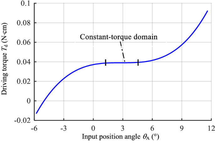

  

  Local zero-stiffness characteristic and constant-torque domain

7 Further Discussion and Experimental Validation

Sections 2 through 7 discuss that the nonlinear characteristic of the crank-slider linkage with springs can be constructed by placing springs at the joint and making the mechanism to work around the right limiting kinematic limb-singularity position (Figure 13(b)). When K_PC ≠ 0, K_RA = K_RB = K_RC, the mechanism exhibits the bi-stable characteristic when works around the right limiting kinematic limb-singularity position which is the unstable equilibrium position. Similarly, for the same springs stiffness, the mechanism produces the bi-stable characteristic when the mechanism moves from the non-singular position and passes the left limiting kinematic limb-singularity position as shown in Figure 16, which must be the unstable equilibrium position. Thus when crank AB fully rotates about pin A, if K_PC ≠ 0, K_RA = K_RB = K_RC = 0, the mechanism exhibits the tri-stable characteristic which has two unstable equilibrium positions being located at the two kinematic limb-singularity positions.

Figure 13

Left limiting kinematic limb-singularity position

However, torsional spring cannot be placed at joints A or B in case of torsional spring failure when crank AB fully rotates about pin A. For pin joint C, it is oscillating during the motion of the mechanism. Therefore, the springs stiffness can be assigned as K_PC ≠ 0, and K_RA = K_RB = 0 to design the tri-stable characteristic, which is shown in Figure 14.

Figure 14

Nonlinear characteristic for different K_RC when K_RA = K_RB = 0 and K_PC = 1 N/cm

Figure 14 shows that when K_PC ≠ 0, and K_RA = K_RB = 0, if K_RC is small, the mechanism generates the tri-stable characteristic. Increment of K_RC decreases the both magnitudes of the first local minimal force and the second maximal force. When K_RC is too great comparing with the translational spring stiffness, K_PC, the driving torque is mainly to resist the torque caused by the torsional spring stiffness, K_RC, the tri-stable characteristic degenerates to the bi-stable characteristic.

It is worth pointed out that the nonlinear characteristic analysis of the mechanism with springs can be used to synthesize the compliant mechanism with nonlinear characteristic. When the mechanism works around one of the two kinematic limb-singularity positions (Figure 3(b) or Figure 13), the nonlinear characteristics can be obtained by the corresponding compliant mechanism based on the rigid-body replacement method. On the other hand, the tri-stable characteristic cannot be obtained by designing the fully compliant mechanism because no compliant rotational joint can fully rotate. However, prismatic joint C and pin joint C can both be replaced by the compliant joints as shown in Figure 15(a), while pin joints A and B are rigid kinematic pairs. Another example is shown in Figure 15(b), where coupler BC is replaced by the lumped-compliant rod and the prismatic joint is replaced by the compound compliant parallelogram mechanism.

Figure 15

Partially compliant crank-slider mechanism

Fragments in-plane thickness of flexures C_i (i = 1, 2, 3) in (Figure 15(a)) and in-plane thickness of rod B_iC_i (i = 1, 2, 3) (Figure 15(b)) can be set to different values to obtain the corresponding equivalent torsional spring stiffness. The equivalent stiffness of compliant rotational joints C and output translational joint can be calculated by referring Ref. [25]. Thus the expected nonlinear stiffness of the mechanism can be designed by assigning appropriate in-plane thickness of the compliant elements.

A symmetrical mechanism with a constant-torque zone was fabricated by slow wire-electrode cutting and assembled as shown in Figure 16 to validate the design of nonlinear stiffness characteristic. It is worth to point out that the constant-torque compliant mechanism can be used in many applications such as the dynamic torque-balancing mechanism [26], knee- and ankle-assisting device [27], and rehabilitating injured human joint [28]. Two types of constant-torque compliant mechanisms were developed in Refs. [29, 30]. But without the 3D printer, it is difficult to machine the two types of compliant mechanisms with complicated curvilinear beams. In this paper, the designed constant-torque compliant mechanism can be manufactured easily. This mechanism, where the rigid crank and the compliant structure are connected by three pin joints, is shown in Figure 16. The structure parameters are given as t = 1 mm, L₁ = 38 mm, L₂ = 30 mm, α = 3°, b₁ = 8 mm, b₂ = 5 mm, and the out-plane thickness of the compliant structure is 5 mm.

Figure 16

Structure parameters of the compliant constant-torque mechanism

According to Ref. [25], the equivalent stiffness of each rotational joint C_i (i = 1, 2, 3) and each translational joint can be obtained by the two following equations

$$K_{\text{RC}} = \frac{2.25EI}{{L_{1} }},\quad K_{\text{P}} = \frac{48EI}{{L_{2} }},$$

where E is the Young’s modulus, and I is the second moment of area about z axis.

We select the spring steel, 85, with Young’s modulus of 200 GPa, as the material of the compliant structure. The experimental testing apparatus is shown in Figure 17, where the rotating platform is applied to rotate the three-jaw chuck that clamps the torque sensor connected to the compliant mechanism. The rotation angle of the mechanism was recorded according by the micrometer, and the driving torque on the compliant mechanism was obtained from the torque sensor.

Figure 17

Experimental testing apparatus

The driving torque can be calculated by Eq. (10), where the geometry parameters can be calculated as

$$\theta_{{{\text{A}}0}} = - \arcsin \frac{{L_{1} \sin \alpha }}{{r_{1} }},r_{ 2} = gL_{ 1} ,e = \, - ( 1- g)L_{ 1} { \sin }a,$$

where γ = 0.85.

We can regard the designed symmetrical compliant mechanism shown in Figure 16 to be the one composed of three crank-slider mechanisms in parallel. Therefore, the driving torque, T, applied on the crank shown in Figure 16 should be three times the toque, T_d, calculated by Eq. (10), namely,

$$T = 3\times T_{\text{d}} .$$

Three curves (torque variation versus the crank rotation angle) corresponding to the PRBM, finite element model and the experimental result are represented in Figure 18. Here the horizontal coordinate, θ, describes the crank rotation angle of the mechanism, which starts form zero, and can be represented below:

$$\theta = \theta_{A} - \theta_{A0} .$$

Figure 18

Comparison of testing result, FEA result and PRBM result

Figure 18 shows that there are errors among the PRBM result, finite element analysis (FEA) and experimental testing result. The error between the PRBM result and the FEA is little, indicating that the PRBM can correctly describe the theoretical model of the compliant mechanism. The relatively large discrepancy between the theoretical model and the experimental result may be due to beam fabrication errors with the available slow wire-electrode system and the assembling tolerance. It indicates that the pseudo-rigid-body model, FEA and experimental result all exhibit the constant-torque characteristic.

8 Conclusions

• (1) A generic method of generating nonlinear characteristics is proposed by using the kinematic limb-singularity positions of the crank-slider linkage with attached springs.

• (2) The mechanism with springs may generate four types of nonlinear characteristics including the bi-stable characteristic, local negative-stiffness characteristic, local zero-stiffness characteristic and positive-stiffness characteristic, when works around and passes the kinematic limb-singularity position. One nonlinear characteristic may transform to another one with different springs stiffness.

• (3) The mechanism only exhibits the positive-stiffness characteristic when moves from the kinematic limb-singularity position.

• (4) When the input crank fully rotates and the two torsional spring stiffness placed at both ends of crank are exclusively zero, for small and great torsional spring stiffness placed at the pin joint connecting the coupler and slider, the mechanism produces the tri-stable characteristic and bi-stable characteristic, respectively.

• (5) The theory of nonlinear stiffness characteristic generation can be used to design compliant mechanisms with nonlinear stiffness characteristic

References

P Lambert, J L Herder. An adjustable constant force mechanism using pin joints and springs. New Trends in Mechanism and Machine Science, 2017, 43: 453–461.
Y S Zheng, Q P Li, B Yan, et al. A Stewart isolator with high-static-low-dynamic stiffness struts based on negative stiffness magnetic springs. Journal of Sound and Vibration, 2018, 422: 390–408.
Z W Yang, C C Lan. An adjustable gravity-balancing mechanism using planar extension and compression springs. Mechanism and Machine Theory, 2015, 92: 314–329.
J J Yu, S S Bi, G H Zong, et al. Kinematics analysis of fully compliant mechanisms using the pseudo-rigid-body model. Journal of Mechanical Engineering, 2002, 38(2): 75–78. (in Chinese)
J J Yu, G B Hao, G M Chen, et al. State-of-art of compliant mechanisms and their applications. Journal of Mechanical Engineering, 2015, 51(13): 53–68. (in Chinese)
Y Q Yu, Q P Xu, P Zhou. New PR pseudo-rigid-body model of compliant mechanisms subject to combined loads. Journal of Mechanical Engineering, 2013, 49(15): 9–14. (in Chinese)
L L Howell. Compliant mechanisms. New York: John Wiley & Sons, 2001.
S P Pellegrini, N Tolou, M Schenk, et al. Bistable vibration energy harvesters: a review. Journal of Intelligent Material Systems and Structures, 2013, 24(11): 1303–1312.
B Andòa, S Baglioa, A R Bulsarab. A bistable buckled beam based approach for vibrational energy harvesting. Sensors and Actuators A: Physical, 2014, 211: 153–161.
N D K Tran, D A Wang. Design of a crab-like bistable mechanism for nearly equal switching forces in forward and backward directions. Mechanism and Machine Theory, 2017, 115: 114–129.
X Liu, F Lamarqe, E Doré, et al. Multistable wireless micro-actuator based on antagonistic pre-shaped double beams. Smart Materials and Structures, 2015, 24: 075028_1-7.
F L Ma, G M Chen. Bi-BCM: A closed-form solution for fixed-guided beams in compliant mechanisms. ASME Journal of Mechanical Design, 2017, 9(1): 014501_1-8.
P B Liu, P Yan. A modified pseudo-rigid-body modeling approach for compliant mechanisms with fixed-guided beam flexures. Mechanical Science, 2017, 8(2): 359–368.
B D Jensen, L L Howell. Bistable configurations of compliant mechanisms modeled using four links and translational joints. ASME Journal of Mechanical Design, 2014, 126(4): 657–666.
S Amine, O Mokhiamar, S Caro. Classification of 3T1R parallel manipulators based on their wrench graph. ASME Journal of Mechanisms and Robotics, 2017, 9(1): 011003_1–10.
A Karimia, M T Masouleha, P CARDOUB. Avoiding the singularities of 3-RPR parallel mechanisms via dimensional synthesis and self-reconfigurability. Mechanism and Machine Theory, 2016, 99: 189–206.
W Ye, Y F Fang, S Guo, et al. Design of reconfigurable parallel mechanisms with discontinuously movable mechanism. Chinse Journal of Mechanical Engineering, 2015, 51(13): 137–143.
R Ranganatha, P S Nairb, T S Mruthyunjaya, et al. A force–torque sensor based on a Stewart Platform in a near-singular configuration. Mechanism and Machine Theory, 2005, 39(9): 971–998.
P Renaud, M Mathelin. Kinematic analysis for a novel design of MRI-compatible torque sensor. IEEE/RSJ International Conference on Intelligent Robots and Systems, October 11-15, 2009, St. Louis, USA: 2640–2646.
B Quentin, V Marc, A Salih. Parallel singularities for the design of softening springs using compliant mechanisms. In ASME International Design Engineering Technical Conferences & Computers and Information in Engineering Conference, August 2-5, 2015, Boston, Massachusetts, USA, DETC2015-47240.
G B Hao, H Y Li, A Nayak, et al. Design of a compliant parallel gripper with multimode jaws. ASME Journal of Mechanisms and Robotics, 2018, 10(3): 031005_1–12.
L Rubbert, S Caro, J Gangloff, et al. Using singularities of parallel manipulators for enhancing the rigid-body replacement design method of compliant mechanisms. ASME Journal of Mechanical Design, 2014, 136(5): 051010_1–9.
M S Baker, L L Howell. On-chip actuation of an in-plane compliant bistable micromechanism. Journal of Microelectromechanical Systems, 2002, 11(5): 566–573.
G B Hao. A framework of designing compliant mechanisms with nonlinear stiffness characteristics. Springer: Microsystem Technologies, 2018, 28(4): 1795–1802.
L L Howell, S P Magleby, B M Olsen. Handbook of compliant mechanisms. New York: John Wiley & Sons, 2013.
V Arakelian, S Ghazaryan. Improvement of balancing accuracy of robotic systems: application to leg orthosis for rehabilitation devices. Mechanism and Machine Theory, 2008, 43(5): 565–575.
S K Agrawal, S K Banala, A Fattah, et al. Assessment of motion of a swing leg and gait rehabilitation with a gravity balancing exoskeleton. IEEE Transactions on Neural Systems and Rehabilitation Engineering, 2007, 15(3): 410–420.
A Kipnis, Y Belman. Constant Torque Range-of-motion Splint. US Patent, 5399154, 1995-03-21.
C W Hou, C C Lan. Functional joint mechanisms with constant-torque outputs. Mechanism and Machine Theory, 2013, 62: 166–181.
H N Prakashah, H Zhou. Synthesis of constant torque compliant mechanisms. ASME Journal of Mechanisms and Robotics, 2016, 8(6): 064503_1-8.
Authors’ contributions
BL and GH in charge of the whole trial, BL wrote the manuscript, GH assisted with sample and laboratory analyses. Both authors read and approved the final manuscript.
Acknowledgements
The authors express their sincere thanks to the referees, and all the members of our discussion group for their beneficial comments.
Authors’ information
Baokun Li, born in 1982, is currently an Associate Professor at Anhui University of Science and Technology, China. He received his PhD degree from Jiangnan University, China, in 2014. His research interests include robotics and mechanisms.
Guangbo Hao, born in 1981, is currently an Associate Professor and a PhD candidate supervisor at University College Cork, Ireland. He received his PhD degree from Heriot-Watt University, United Kingdom, in 2011. His research interests include robotics and mechanisms.
Competing interests
The authors declare that they have no competing interests.
Funding
Supported by National Natural Science Foundation of China (Grant No. 51605006), and Research Foundation of Key Laboratory of Manufacturing Systems and Advanced Technology of Guangxi Province, China (Grant No. 17-259-05-013K).
Author information
Authors and Affiliations
Corresponding author
Rights and permissions
Open Access This article is distributed under the terms of the Creative Commons Attribution 4.0 International License (http://creativecommons.org/licenses/by/4.0/), which permits unrestricted use, distribution, and reproduction in any medium, provided you give appropriate credit to the original author(s) and the source, provide a link to the Creative Commons license, and indicate if changes were made.
About this article
Cite this article
Li, B., Hao, G. On Generating Expected Kinetostatic Nonlinear Stiffness Characteristics by the Kinematic Limb-Singularity of a Crank-Slider Linkage with Springs. Chin. J. Mech. Eng. 32, 54 (2019). https://doi.org/10.1186/s10033-019-0369-z
Received:
Accepted:
Published:
DOI: https://doi.org/10.1186/s10033-019-0369-z