- Original Article
- Open access
- Published:
An Interpretable Denoising Layer for Neural Networks Based on Reproducing Kernel Hilbert Space and its Application in Machine Fault Diagnosis
Chinese Journal of Mechanical Engineering volume 34, Article number: 44 (2021)
Abstract
Deep learning algorithms based on neural networks make remarkable achievements in machine fault diagnosis, while the noise mixed in measured signals harms the prediction accuracy of networks. Existing denoising methods in neural networks, such as using complex network architectures and introducing sparse techniques, always suffer from the difficulty of estimating hyperparameters and the lack of physical interpretability. To address this issue, this paper proposes a novel interpretable denoising layer based on reproducing kernel Hilbert space (RKHS) as the first layer for standard neural networks, with the aim to combine the advantages of both traditional signal processing technology with physical interpretation and network modeling strategy with parameter adaption. By investigating the influencing mechanism of parameters on the regularization procedure in RKHS, the key parameter that dynamically controls the signal smoothness with low computational cost is selected as the only trainable parameter of the proposed layer. Besides, the forward and backward propagation algorithms of the designed layer are formulated to ensure that the selected parameter can be automatically updated together with other parameters in the neural network. Moreover, exponential and piecewise functions are introduced in the weight updating process to keep the trainable weight within a reasonable range and avoid the ill-conditioned problem. Experiment studies verify the effectiveness and compatibility of the proposed layer design method in intelligent fault diagnosis of machinery in noisy environments.
1 Introduction
In practical engineering, gears, shafts, bearings, and other key components in rotating machinery frequently occur various failures due to severe work conditions such as alternating load and long operational time [1, 2]. To capture such failures before disasters, developing timely and accurate fault diagnosis methods for rotating machinery is important. In recent decades, with the rapid development of sensor technology and data-driven techniques, intelligent machine health monitoring methods based on machine learning have become an important research field in engineering [3,4,5]. As a dominating branch of machine learning, deep learning methods manage to utilize deep architectures with stacked layers to extract essential features hidden in data and achieve excellent prediction performance [6]. Some commonly used deep learning architectures, such as deep belief networks (DBNs) [7, 8], deep auto-encoders (DAEs) [9,10,11], and convolutional neural networks (CNNs) [12,13,14], have been successfully applied in machine fault diagnosis. Unfortunately, when the actual data acquisition environment becomes complicated and uncontrollable, the sampling data are inevitably mixed with noise, which may pose challenges to reliable feature extractions and increase the risk of overfitting. Therefore, it is crucial to develop effective methods to eliminate the effects of noise and improve the accuracy of feature extraction and fault diagnosis.
In recent years, the challenge introduced by noise for deep learning has attracted widespread attention from scholars, and the corresponding solution can be roughly divided into two categories according to whether it modifies the original network structure. Techniques entailing no network structure modifications, such as the signal preprocessing based denoising method, are successfully applied in fault diagnosis of rotating machinery [15, 16]. Instead of the raw signal, the data processed by signal analysis techniques, such as the wavelet transform, are applied to fit the deep neural network model. However, since parameters used in signal processing methods are dependent on noise whose properties are hard to obtain, the selection of parameters has become an obstacle. Using extra noise to train deep neural networks is another denoising method eliminating the need for network structure modifications [17], where the input is taken as the clean signal mixed with the well-designed noise similar to the practical environment noise, while the output is taken as the original clean signal. Via unsupervised learning like DAE, this method can robustly extract hierarchical features for further classification or regression. However, this method requires clean signals obtained in advance, which is extremely difficult to achieve in practical engineering. Another popular denoising method is to modify the network structure and using the raw data to fit it, where techniques to prevent overfitting, such as dropout in DAE [18] and pooling in CNN [19], have been widely applied in various noisy working conditions [20, 21]. These techniques can be interpreted as reducing the complex co-adaptation between neurons and following the idea of biological evolution [22]. However, its physical interpretability is not as sufficiently rigorous as that of conventional machine learning methods. Moreover, the selection of hyper-parameters, such as the keep-probability of dropout, still haunts users. Designing dedicated neural networks is another way to achieve noise reduction by modifying the network structure. For example, adding the residual building units to CNN is one of the relatively new methods that has been proven to improve the accuracy of the classification task [23]. However, the complicated network design also introduces a vast number of parameters to the network model and increases the risk of overfitting. Meanwhile, the special network structure design undermines its compatibility with different networks.
Considering the excellent interpretability of classical data preprocessing methods and the self-adaption of network modeling strategies, combing the classical data processing methods as a part of the neural network has been regarded as an effective and well-interpreted method [24]. Through the backpropagation of the neural network, parameters of the classical data processing method can be adaptively estimated without manual intervention. Besides, the original physical interpretability of the classical approach is also retained. Among various classical data processing approaches, using the representation theory to solve the regularization problem in the reproducing kernel Hilbert space (RKHS) is an effective denoising method. Few parameters and multiple kernel choices render this approach widely applicable [25, 26]. Faced with the dilemma of the current denoising method for neural networks, we proposed a novel, well-compatible, and well-interpreted denoising layer based on RKHS in this paper. By analyzing the regularization problem in RKHS, the parameter that controls the system bandwidth and the signal smoothness is chosen as the only trainable parameter of the proposed layer. Due to this few-parameter layer design, the overfitting problem of the whole network can be alleviated. Meanwhile, based on the derivation of the forward and backward propagation of the proposed denoising layer, this only trainable parameter can be adaptively adjusted to fit the noise level of the original noisy data. Moreover, since the size of the denoised data is the same as that of the raw data, the established denoising layer can be conveniently embedded into various neural networks like DBN and CNN. The experimental studies in Section 5 verify the effectiveness of the novel denoising layer in improving identification accuracy.
The remainder of the paper is as follows. In Section 2, we briefly introduce the theoretical basis of the RKHS based denoising method. The forward and backward propagation of the proposed denoising layer is presented in Section 3, and machine fault diagnosis using the interpretable denoising layer is presented in Section 4. In Section 5, the experimental studies demonstrate the effectiveness and compatibility of the proposed method. Conclusions are given in Section 6.
2 RKHS Based Denoising Method
Given a finite number of noisy time-series samples \(D = \{ t_{i} ,x_{i} \}_{i = 1}^{l}\), the functional relation \(f\) between time step \(t_{i}\) and \(x_{i}\) can be approximated by minimizing the regularization problem as
where the regularization term \(\left\| f \right\|_{{\varvec{K}}}^{2}\) is a norm in RKHS \({\mathcal{H}}\), which is induced by the symmetric positive definite kernel K, and \(\lambda\) is the corresponding regularization parameter. By introducing the regularization term that includes the prior knowledge of the solution, the smoothness of the mapping function \(f\) can be controlled so that the undesired behaviors can be penalized [27]. Using different kernels, we can get various regularization tasks. In this paper, the Gaussian kernel is chosen due to its conciseness and universality, which is defined as
where \(\sigma\) is a hyperparameter in this kernel function, which denotes the standard deviation of the Gaussian function and controls the smoothness of the kernel.
According to the representer theorem [28], the mapping function \(f\) is effectively constricted in the RKHS \({\mathcal{H}}\) induced by K, and the minimizer of the regularization problem can be formulated as
where \(\cdot\) represents the dot product, \({\varvec{K}}(t)\) is the vector of functions defined as \(({\varvec{K}}(t))_{i} = K(t,t_{i} )\), and c is the corresponding vector of coefficients defined as \(({\varvec{c}})_{i} = c_{i}\). The relationship between x and c can be represented as
where the matrix K and the vector x are defined as \(({\varvec{K}})_{ij} = K(t_{i} ,t_{j} )\) and \(({\varvec{x}})_{i} = x_{i}\), respectively, and I denotes an \(l \times l\) identity matrix.
According to Eqs. (3) and (4), the denoised time-series can be represented as
where the vector \({\varvec{b}}(t)\) of the basis functions is defined as
Two parameters \(\sigma\) and \(\lambda\) are to be determined in the basis functions \({\varvec{b}}(t)\) as well as the related function \(f(t)\). To clarify the effects of two parameters on the denoising process, we conduct a set of tests for variable analysis, including four cases with different \(\lambda\) and three cases with different \(\sigma^{2}\). In these tests, the kernel size and the adjacent time step interval are set as 500 × 500 and 1, respectively. The impulse signal impacts the system at the 250th time step, and the corresponding impulse response is shown in Figure 1.

Influences of \(\sigma\) and \(\lambda\) on \(f\) when the system is excited by an impulse signal: a \(\sigma^{2} = 1\), b \(\sigma^{2} = 10\), and c \(\sigma^{2} = 100\)
From Figure 1, it is clear to see that this denoising method acts as a low-pass filter. Changes in either one of the two parameters can dynamically adjust the system bandwidth and make the system response \(f(t)\) sharper or smoother. Considering the complexity of subsequent calculations, the regularization parameter \(\lambda\) is chosen as the only trainable variable to control the system bandwidth changes. Meanwhile, to ensure the denoising system has optimal dynamic adjustable range via changing \(\lambda\), the fixed value of \(\sigma\) should also have specific constraint rules. When \(\sigma\) is fixed at a small value, as shown in Figure 1(a), the system is equivalent to a filter with a low quality factor, which greatly affects the frequency resolution capability of the system. When \(\sigma\) is fixed at a large value, as shown in Figure 1(c), the system more like an ideal filter, but it is hard to change the system bandwidth by adjusting the parameter \(\lambda\). In order to make the RKHS based denoising method have adequate performance in bandwidth control, the fixed value of \(\sigma\) can be determined by cross-validation so that the adjustable bandwidth range of the system is balanced with the quality factor.
3 Interpretable Denoising Layer Design for Neural Networks
3.1 Forward Propagation of the Denoising Layer
To reduce the effect of noise, we propose a novel interpretable denoising layer based on RKHS in front of the traditional neural networks. According to Eqs. (5) and (6), given the noisy input signal x with length L, the forward mapping of the denoising layer in the entire network can be written as
where the output vector z indicates the denoised signal, and z has the same length as the original input signal x. By connecting with the subsequent network layer, the only trainable parameter \(\lambda\) in this layer can be adaptively adjusted in the entire network. The regularization parameter \(\lambda\) should always be kept positive. Meanwhile, the proposed denoising system bandwidth will change slower and slower as the parameter increases. To ensure that the system bandwidth changes within a reasonable range, the exponent function and power function are adopted to express the parameter \(\lambda\) as
where \(\gamma\) is the trainable parameter actually used in the neural network, and \(\alpha\) is a power term that further balance the relationship between the speed and the range of change of \(\gamma\).
3.2 Backpropagation of the Denoising Layer
Generally, in the training process of stacked neural networks, an iterative gradient-based backpropagation is used to solve the optimization problem. In order to make the proposed noise reduction layer compatible with the standard networks, it is necessary to use a similar technique to update the weights of the proposed noise reduction layer. Since the proposed denoising layer is set as the first layer of the whole network, only the trainable parameter \(\gamma\) needs to be updated. The gradient \(\delta_{\gamma }\) of \(\gamma\) can be calculated as
where \(J\) denotes the loss of the entire network, \(\partial\) denotes the derivative operator, and the matrix T is defined as
In practical applications, we notice that a small learnable parameter \(\gamma\) will cause the ill-conditioned problem for the inversion of T. To overcome this obstacle, the updated value of the trainable parameter is restricted within a reasonable range by introducing a piecewise function
where \(\gamma_{t}\) denotes the infimum that meets the calculation accuracy requirement of the inverse matrix \({\varvec{T}}^{ - 1}\), \(\delta\) denotes the gradient actually used during the update process, and \(\eta\) denotes the learning rate, which is a positive scalar that determines the size of the gradient update step.
4 Machine Fault Diagnosis with the Denoising Layer
4.1 Deep Neural Networks Based Fault Diagnosis
Unlike traditional data-driven methods in which the manual design and feature extraction are needed [29, 30], deep learning using neural networks offers a powerful and effective solution without hand-crafted features for machine fault diagnosis. In a fault classification task with m categories, by building neural networks with n hidden layers of transformations, the hierarchical feature behind the machinery data can be extracted and represented as
where the m-dimensional feature vector h is defined as \(({\varvec{h}})_{i} = h_{i}\), and \(\phi^{(i)}\) is used for the mapping of the ith hidden layer, such as the linear combination with a nonlinear activation function or the convolution operation. To normalize the learned features to a probability distribution over predicted output classes, a softmax function \(p_{i}\) is added to the end of the stacked network, and \(p_{i}\) is defined as
where the m-dimensional feature vector h is mapped into an m-dimensional output vector p. p is formulated by \(\sum\nolimits_{i} {p_{i} = 1}\). To evaluate the performance of the classifier, the cross-entropy \(J\) is used as the loss function, which is defined as
where \(y_{c}\) represents the target probability of the occurrence of the cth fault type. If the sample belongs to the cth fault type, \(y_{c}\) is set as 1. Otherwise, \(y_{c}\) is set as 0. Through the backpropagation algorithm based on the gradients updating, the value of the loss function \(J\) decreases until the network has the optimal recognition performance.
4.2 Procedure of Fault Diagnosis Using the Denoising Layer
Combined with the proposed interpretable denoising layer, the entire procedure for intelligent fault diagnosis of the machinery in noisy environments can be summarized as follows.
-
(1)
Data Acquisition
Use sensors and data acquisition equipment to collect the original time-domain vibration signals and the corresponding state labels of the machine to be diagnosed in the running state.
-
(2)
Data Preprocessing
Split the original signal into data segments of equal length, and standardize the data samples as inputs of the network. Use the one-hot encoding to indicate the state labels of the machine as outputs of the network. Randomly divide the processed samples into the training, validation, and test sets, respectively.
-
(3)
Backbone Preparation
According to the characteristics of the signal to be analyzed, select an appropriate stack neural network, such as DBN and CNN as the backbone model, where the input layer size of the network should be the same as the input sample. According to the number of fault categories, set the softmax layer as the last layer and determine the cross-entropy loss function as the objection function via Eqs. (13) and (14).
-
(4)
Denoising Layer Design
Design the interpretable denoising layer that matches the size of the input sample, and then perform the forward and backward propagation algorithms as specified in Eqs. (7)‒(11).
-
(5)
Model Combination
Prefix the proposed interpretable denoising layer to the selected backbone network to construct the combined denoising neural network.
-
(6)
Model Training and Validation
Train the combined network with the training dataset. Update the proposed denoising layer via Eqs. (9)‒(11), and use the backpropagation algorithm to update the remaining layers. Utilize the validation dataset to evaluate the training performance of the denoising network, and choose the network framework with the lowest validation loss to predict the fault category to be assessed with the test dataset.
To illustrate the above machine fault diagnosis procedure, the whole algorithm is summarized in Figure 2.

General procedure of machine fault diagnosis
5 Experiment and Analysis
To validate the proposed denoising layer for machinery fault diagnosis, the proposed interpretable denoising layer is embedded in the standard neural networks to conduct fault diagnosis for the following two systems.
5.1 Fault Diagnosis of Rolling Bearing
In this subsection, the original experimental vibration data are obtained from the rolling bearing fault data acquisition experimental bench of the Bearing Data Center in Case Western Reserve University (CWRU) [31], as shown in Figure 3. The required data are collected by accelerometers and the digital audio tape recorder at the driven end of the motor housing. The sampling frequency is set as 48 kHz. Under this sampling frequency, the available data include three bearing fault types: inner race pitting, ball pitting, and outer race pitting. Each type of fault has different degrees of damage. In order to balance the proportion of various types of datasets, we select datasets with similar data lengths. Each set contains two subsets corresponding to two damage levels for each failure. In the selected datasets, pits with diameters of 0.007 inches and 0.021 inches represent the minor fault and the serious fault, respectively. Therefore, six fault conditions are considered in this validation experiment in total, and the details of all the used datasets are described in Table 1.

Configuration of the experimental system used by CWRU
To further illustrate the effects of noise on identification, an additional Gaussian white noise with zero mean is added to the original dataset. The signal to noise ratio (SNR) of the noise is set to 10 dB, 5 dB, 0 dB, and − 5 dB, respectively. Together with the original datasets, a total of five types of datasets with different noise levels are analyzed in the following experiments.
For data preparation, all the datasets are resampled using 500-point. Since the original length of the dataset, each type of fault corresponds to 300 samples, 1800 samples are used in this experiment in total, where the numbers of training samples, verification samples, and test samples are set to 1000, 300, and 500, respectively. Besides, during the training process of the following DBN based model, these samples are standardized.
-
(1)
DBN with the Denoising Layer
In this subsection, the DBN model, which leads to the revolution of deep learning, is applied as the backbone and competitive method of the proposed denoising layer. As an essential part of DBN, the restricted Boltzmann machine (RBM) is a special undirected probability graph model that includes a visible layer and a hidden layer. Its weights and biases can be obtained through unsupervised learned with the contrast divergence algorithm [32]. By stacking RBMs, the hidden layer of the former RBM is regarded as the visible layer of the latter RBM, and then a deep network with trainable parameters that can be pre-trained is formed. In this experiment, as shown in Figure 4, the DBN is stacked by four RBMs, and unit numbers of all the hidden layers are set as 180, 60, 20, 6, respectively.
Figure 4 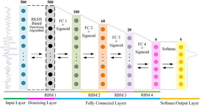
DBN based structure applied to the experiment
Generally, the RBM is designed for binary visible and hidden units. However, in this task, the probability distribution ability of the RBM on real value is required. To address this issue, the Gaussian-Bernoulli RBM (GBRBM) [33] is utilized to pre-train the first hidden layer of the entire DBN, while the standard Bernoulli-Bernoulli RBM (BBRBM) [6] is used to pre-train the other layers. After pre-training each individual RBM, the proposed denoising layer is added in front of the network, and the layers of the entire neural network need to be further fine-tuned for classification by the backpropagation algorithm. To conveniently calculate the denoising algorithm and ensure the trainable parameters have a good performance, the unit time step interval is applied in Eq. (2), and the associated variance \(\sigma^{2}\) is chosen as 10. Besides, the parameter \(\alpha\) formed in Eq. (8) and the infimum \(\gamma_{t}\) used in Eq. (11) are set as 3 and \(- 3\), respectively. For classification, the softmax layer is added to the end of the stacked network, and the cross-entropy in Eq. (14) is used as the loss function. The Adam optimizer is used in the fine-tuning of the network, and the maximum training epoch is 1000. Table 2 lists the five average test results, corresponding to five noise levels. Besides, the test results estimated by the DBN without the denoising layer are also listed in this table.
Table 2 Classification accuracy of the DBN based experiment (%) According to the test results, the classification accuracy of the network decreases in the presence of noise. When noise with the SNR being − 5 dB is mixed into the original dataset, the classification accuracy of the competitive DBN is reduced to half of the original. Compared with the competitive DBN, the DBN with the proposed denoising layer can efficiently improve the classification accuracy. In the presence of strong noise, adding the denoising layer can increase the accuracy by 10% at most. Figure 5 indicates the variance in validation loss during the training process. Obviously, the proposed network can make the validation loss reach a smaller cross-entropy loss. When stronger noise is mixed into the data, the loss difference between the proposed DBN and the competitive DBN is more significant.
Figure 5 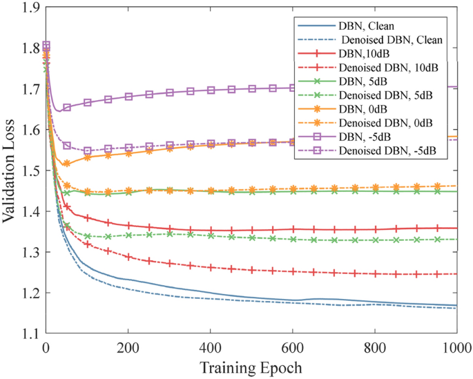
Variance of the validation loss based on DBN
-
(2)
CNN with the Denoising Layer
CNN is an important branch of deep neural networks and has shown its success in various applications, including machine fault diagnosis. According to the application of spatially shared weights and the pooling layers, the parameters in CNN are much fewer than the typical full connected network and make the model more robust. Besides, the one-dimensional CNN (1d-CNN) has been shown to have similar properties to Fourier transform, which helps the network extract the frequency features from the time sequence and thus is beneficial to the fault diagnosis. Hence, this following experiment uses a 1d-CNN as another backbone of the proposed denoising method.


The applied network architecture in detail is shown in Figure 6, which consists of two combined blocks that are composed of a convolutional layer and a max-pooling layer to learn features. Six convolution filters with a length of four points exist in the first combined block, and the pooling size of the max-pooling operation is set as 15. In the second combined block, the length of the convolutional filter and the pooling size remain unchanged, while the number of filters is increased to 12. Meanwhile, the zero-padding is used in the convolution operation, ensuring that the signal length before and after the procedure remains the same. After learning features, the output is flattened and then sent into a full-connected layer. As before, the softmax layer is added to the end of the whole network for classification, and the cross-entropy defined in Eq. (14) is used.

CNN based structure applied to the experiment
The proposed denoising layer is added in front of the network, where the parameters used to calculate the kernel and propagation remain unchanged. After that, the whole network is trained using the backpropagation algorithm. The Adam optimization is still applied, and the maximum training epoch is set as 1000. The five average test results, corresponding to five noise levels, are listed in Table 3. For comparison, the test results estimated by the competitive CNN without the denoising layer are also listed in this table. Meanwhile, the variance in validation loss during the training process is shown in Figure 7.

Variance of the validation loss on the bearing dataset based on CNN
The experimental results show that compared with DBN, CNN has better classification performance in fault diagnosis. For the dataset without additional noise, the proposed denoising layer improves the classification accuracy of the network by 0.44%. In fact, thanks to the advantages of weight sharing and pooling, the classification accuracy of the original CNN is already high, so the proposed noise reduction method has little room for further improvement in accuracy. Nevertheless, in the presence of strong noise, the classification accuracy is still increased by nearly 4% with the aid of the proposed denoising layer. Meanwhile, Figure 7 shows that the proposed network can reduce the validation loss just as demonstrated in the last experiment. According to the experimental results of DBN and CNN, the proposed denoising layer can be considered as an effective and compatible neural network.
5.2 Fault Diagnosis of Planetary Gearbox
To further verify the feasibility and applicability of the proposed method, the proposed denoising layer is applied to a planetary gearing system. The experimental setup is shown in Figure 8. In this experiment, a planetary gearbox whose components can be replaced is set up in a simple drive system, and the accelerometer is fixed on the cage of the gearbox to sample the required data. The measurements can be further fed into the computer via a data acquisition card, and the sampling frequency is set as 10.24 kHz. As shown in Figure 9, four types of designed faults are considered, which include tooth fractures of three different gears and the outer race pitting of the rolling bear. Five corresponding health conditions considered in this case are listed in Table 4, which indicates the normal state, the single fault, the double fault, the triple fault, and the compound fault of the gear and rolling bearing, respectively.

Configuration of the experimental planetary gearing system

Defective component of the experimental planetary gearing system: a tooth fracture of the ring gear, b tooth fracture of the sun wheel, c tooth fracture of the planetary gear, and d outer race pitting of the rolling bearing
As before, an additional Gaussian white noise with zero mean is added to the original dataset to demonstrate the effects of noise on identification, where the SNR of the noise is set to 10 dB. Thus, two types of datasets with different noise levels are analyzed in the following experiments. For data preparation, the datasets are divided into 500-point samples as before, and each health condition corresponds to 1000 samples. Thus, a total of 5000 samples are used, where numbers of training, verification, and test samples are set to 3000, 1000, and 1000, respectively.
The 1d-CNN model is used as the backbone and also the competitive method of the proposed denoising approach. The only difference between the network structure used here and the 1d-CNN used in Section 5.1 is the number of units of the fully connected layer and the softmax layer, which has changed from six to five. Other hyperparameters, including the parameters controlling the training process, remain changed. The average results of five tests using the original and improved CNN models, corresponding to two noise levels, are listed in Table 5, and the variation in validation loss using two models during the training process is shown in Figure 10.

Variance of the validation loss on the planetary gearbox dataset based on CNN
According to the above results, the dataset mixed with additional noise affects the classification accuracy of the network in a similar manner as before. Compared with the original CNN model, the network with the proposed denoising layer still helps in the minimization of the validation loss. Besides, whether or not additional noise is added into the dataset, the classification accuracy of the network can be increased by more than 2% with the aid of the denoising layer. In the presence of the additional noise, the proposed layer helps the network increase classification accuracy more significantly. Thus far, the effectiveness of the proposed denoising layer in practical application has been well demonstrated.
6 Conclusions
In the present study, based on the regularization in RKHS, a novel interpretable denoising layer is proposed as the first layer of a standard neural network to reduce the effect of noise on prediction results. (1) By analyzing the influencing mechanism of parameters in the regularization process in RKHS, the parameter with the low computational cost and clear physical meaning for denoising is selected as the only trainable parameter of this layer. (2) The forward and backward propagation algorithms of the proposed layer are proposed, which ensure not only the adaptability of the trainable parameter updates, but also the compatibility of the denoising layer with various network structures. (3) The procedure of mechanical fault diagnosis using the denoising layer is summarized, and experimental studies further show that the proposed novel denoising method is well compatible with various networks and greatly helps in practical fault diagnosis in noisy environments.
On the other hand, the proposed method still has the limitation in selecting the kernel function reasonably according to the size and dimensions of samples. In fact, this limitation plagues all kernel-based regression methods, and the hybrid kernel function is expected to become an innovative solution. The authors will continue to research this topic in the future.
References
L Lin, C F Hu. HHT-based AE characteristics of natural fatigue cracks in rotating shafts. Mechanical Systems and Signal Processing, 2012, 26: 181–189.
J R Stack, T G Habetler, R G Harley. Fault classification and fault signature production for rolling element bearings in electric machines. IEEE Transactions on Industry Applications, 2004, 40(3): 735-739.
Y Lei, B Yang, X Jiang, et al. Applications of machine learning to machine fault diagnosis: A review and roadmap. Mechanical Systems and Signal Processing, 2020, 138: 106587.
X Dai, Z Gao. From model, signal to knowledge: A data-driven perspective of fault detection and diagnosis. IEEE Transactions on Industrial Informatics, 2013, 9 (4): 2226-2238.
R Zhao, R Yan, Z Chen, et al. Deep learning and its applications to machine health monitoring. Mechanical Systems and Signal Processing, 2019, 115: 213-237.
G E Hinton, R R Salakhutdinov. Reducing the dimensionality of data with neural networks. Science, 2006, 313(5786): 504-507.
H Shao, H Jiang, H Zhang, et al. Electric locomotive bearing fault diagnosis using a novel convolutional deep belief network. IEEE Transactions on Industrial Electronics, 2017, 65(3): 2727-2736.
H Shao, H Jiang, X Zhang, et al. Rolling bearing fault diagnosis using an optimization deep belief network. Measurement Science and Technology, 2015, 26(11): 115002.
F Jia, Y Lei, L Guo, et al. A neural network constructed by deep learning technique and its application to intelligent fault diagnosis of machines. Neurocomputing, 2018, 272: 619-628.
W Sun, S Shao, R Zhao, et al. A sparse auto-encoder-based deep neural network approach for induction motor faults classification. Measurement, 2016, 89: 171-178.
X Wu, Y Zhang, C Cheng, et al. A hybrid classification autoencoder for semi-supervised fault diagnosis in rotating machinery. Mechanical Systems and Signal Processing, 2021, 149: 107327.
T Ince, S Kiranyaz, L Eren, et al. Real-time motor fault detection by 1-D convolutional neural networks. IEEE Transactions on Industrial Electronics, 2016, 63(11): 7067-7075.
X Ding, Q He. Energy-fluctuated multiscale feature learning with deep convnet for intelligent spindle bearing fault diagnosis. IEEE Transactions on Instrumentation and Measurement, 2017, 66(8): 1926-1935.
F Jia, Y Lei, N Lu, et al. Deep normalized convolutional neural network for imbalanced fault classification of machinery and its understanding via visualization. Mechanical Systems and Signal Processing, 2018, 110: 349-367.
Y Han, B Tang, L Deng. Multi-level wavelet packet fusion in dynamic ensemble convolutional neural network for fault diagnosis. Measurement, 2018, 127: 246-255.
W Sun, B Yao, N Zeng, et al. An intelligent gear fault diagnosis methodology using a complex wavelet enhanced convolutional neural network. Materials, 2017, 10(7): 790.
X Liu, Q Zhou, J Zhao, et al. Fault diagnosis of rotating machinery under noisy environment conditions based on a 1-D convolutional autoencoder and 1-D convolutional neural network. Sensors, 2019, 19(4): 972.
P Vincent, H Larochelle, Y Bengio, et al. Extracting and composing robust features with denoising autoencoders. Proceedings of the 25th International Conference on Machine Learning, 2008: 1096-1103.
C-Y Lee, P W Gallagher, Z Tu. Generalizing pooling functions in convolutional neural networks: Mixed, gated, and tree. Artificial Intelligence and Statistics, 2016: 464-472.
C Lu, Z-Y Wang, W-L Qin, et al. Fault diagnosis of rotary machinery components using a stacked denoising autoencoder-based health state identification. Signal Processing, 2017, 130: 377-388.
B Ma, H Hu, J Shen, et al. Generalized pooling for robust object tracking. IEEE Transactions on Image Processing, 2016, 25(9): 4199–4208.
A Krizhevsky, I Sutskever, G E Hinton. Imagenet classification with deep convolutional neural networks. Advances in Neural Information Processing Systems, 2012: 1097-1105.
M Zhao, S Zhong, X Fu, et al. Deep residual shrinkage networks for fault diagnosis. IEEE Transactions on Industrial Informatics, 2019, 16(7): 4681-4690.
T Li, Z Zhao, C Sun, et al. Adaptive channel weighted CNN with multi-sensor fusion for condition monitoring of helicopter transmission system. IEEE Sensors Journal, 2020, 99: 1.
G Pillonetto, F Dinuzzo, T Chen, et al. Kernel methods in system identification, machine learning and function estimation: A survey. Automatica, 2014, 50(3): 657-682.
P Bouboulis, K Slavakis, S Theodoridis. Adaptive kernel-based image denoising employing semi-parametric regularization. IEEE Transactions on Image Processing, 2010, 19(6): 1465-1479.
T Evgeniou, M Pontil, T Poggio. Regularization networks and support vector machines. Advances in Computational Mathematics, 2000, 13(1): 1.
B Schölkopf, R Herbrich, A J Smola. A generalized representer theorem. International Conference on Computational Learning Theory, 2001: 416-426.
G Tu, X Dong, S Chen, et al. Iterative nonlinear chirp mode decomposition: A Hilbert-Huang transform-like method in capturing intra-wave modulations of nonlinear responses. Journal of Sound and Vibration, 2020, 485: 115571.
G Tu, X Dong, C Qian, et al. Intra-wave modulations in milling processes. International Journal of Machine Tools and Manufacture, 2021: 103705.
Case Western Reserve University Bearing Data Center, [online]. Available: http://csegroups.case.edu/bearingdatacenter/pages/downloaddata-file.
G E Hinton, S Osindero, Y-W Teh. A fast learning algorithm for deep belief nets. Neural Computation, 2006, 18(7): 1527-1554.
G Hinton. A practical guide to training restricted Boltzmann machines. Momentum, 2010, 9: 1.
Acknowledgements
Not applicable.
Funding
Supported by National Natural Science Foundation of China (Grant Nos. 12072188, 11632011, 11702171, 11572189, 51121063), and Shanghai Municipal Natural Science Foundation of China (Grant No. 20ZR1425200).
Author information
Authors and Affiliations
Contributions
BZ took most of the research work, including the literature research, modeling, results analysis, and paper writing. CC and ZP are supervisors who provided the opportunity for cooperative research and offered the original idea for the paper. GT, QH, and GM assisted with the results analysis and paper revision. All authors read and approved the final manuscript.
Authors’ Information
Baoxuan Zhao, born in 1995, is currently a Ph.D. candidate at State Key Laboratory of Mechanical System and Vibration, Shanghai Jiao Tong University, China. He received his B.S. degree from Shandong University, China, in 2017. His research interests include nonlinear vibration, intelligent monitoring, and fault diagnosis for machines and structures.
Changming Cheng, born in 1987, is currently an assistant professor at State Key Laboratory of Mechanical System and Vibration, Shanghai Jiao Tong University, Shanghai, China. He received his Ph.D. degree from Shanghai Jiao Tong University, China, in 2015. His research interests include signal processing, nonlinear system identification, machine health diagnosis, and prognostics.
Guowei Tu, born in 1998, is currently a master candidate at State Key Laboratory of Mechanical System and Vibration, Shanghai Jiao Tong University, China. He received his B.S. degree from Chongqing University, China, in 2019. His research interests include nonlinear vibration and signal processing.
Zhike Peng, born in 1974, is currently a Changjiang distinguished professor at State Key Laboratory of Mechanical System and Vibration, Shanghai Jiao Tong University, China. He received his Ph.D. degree from Tsinghua University, China, in 2002. His current research interests include nonlinear vibration, signal processing and condition monitoring, and fault diagnosis for machines and structures.
Qingbo He, born in 1980, is currently a professor at State Key Laboratory of Mechanical System and Vibration, Shanghai Jiao Tong University, China. He received his Ph.D. degree from University of Science and Technology of China, China, in 2007. His current research interests include a combination of vibration analysis, signal processing, and metamaterials design for intelligent monitoring, diagnosis, and control in complex machines.
Guang Meng, born in 1961, is currently a professor at State Key Laboratory of Mechanical System and Vibration, Shanghai Jiao Tong University, China. He received his Ph.D. degree from Northwestern Polytechnical University, China, in 1988. His research interests include dynamics and vibration control of mechanical systems, nonlinear vibration, and microelectromechanical systems.
Corresponding author
Ethics declarations
Competing Interests
The authors declare no competing financial interests.
Rights and permissions
Open Access This article is licensed under a Creative Commons Attribution 4.0 International License, which permits use, sharing, adaptation, distribution and reproduction in any medium or format, as long as you give appropriate credit to the original author(s) and the source, provide a link to the Creative Commons licence, and indicate if changes were made. The images or other third party material in this article are included in the article's Creative Commons licence, unless indicated otherwise in a credit line to the material. If material is not included in the article's Creative Commons licence and your intended use is not permitted by statutory regulation or exceeds the permitted use, you will need to obtain permission directly from the copyright holder. To view a copy of this licence, visit http://creativecommons.org/licenses/by/4.0/.
About this article

Cite this article
Zhao, B., Cheng, C., Tu, G. et al. An Interpretable Denoising Layer for Neural Networks Based on Reproducing Kernel Hilbert Space and its Application in Machine Fault Diagnosis. Chin. J. Mech. Eng. 34, 44 (2021). https://doi.org/10.1186/s10033-021-00564-5
Received:
Revised:
Accepted:
Published:
DOI: https://doi.org/10.1186/s10033-021-00564-5