Acceleration-Dependent Analysis of Vertical Ball Screw Feed System without Counterweight

Abstract

The distinguishing feature of a vertical ball screw feed system without counterweight is that the spindle system weight directly acts on the kinematic joints. Research into the dynamic characteristics under acceleration and deceleration is an important step in improving the structural performance of vertical milling machines. The magnitude and direction of the inertial force change significantly when the spindle system accelerates and decelerates. Therefore, the kinematic joint contact stiffness changes under the action of the inertial force and the spindle system weight. Thus, the system transmission stiffness also varies and affects the dynamics. In this study, a variable-coefficient lumped parameter dynamic model that considers the changes in the spindle system weight and the magnitude and direction of the inertial force is established for a ball screw feed system without counterweight. In addition, a calculation method for the system stiffness is provided. Experiments on a vertical ball screw feed system under acceleration and deceleration with different accelerations are also performed to verify the proposed dynamic model. Finally, the influence of the spindle system position, the rated dynamic load of the screw-nut joint, and the screw tension force on the natural frequency of the vertical ball screw feed system under acceleration and deceleration are studied. The results show that the vertical ball screw feed system has obviously different variable dynamics under acceleration and deceleration. The influence of the rated dynamic load and the spindle system position on the natural frequency under acceleration and deceleration is much greater than that of the screw tension force.

1 Introduction

The ball screw is widely used in the X, Y, and Z axes of high-speed and high-precision machine tools; its importance is self-evident. Its dynamic characteristics directly affect the fatigue life of the mechanism, the bandwidth of the servo system [1,2,3], the positioning accuracy of the machine tool [4,5,6,7], and the machining stability [8, 9]. Therefore, studies on its system dynamics have received increasing attention.

A ball screw is used in the horizontal axis of machine tools and directly links the worktable and the bed. The position of the screw-nut joint and the speed and acceleration of the ball screw feed system affect the dynamic characteristics of the worktable. Wang et al. [10] proposed a three-dimensional mechanical model of a twin ball screw-driven table to predict the vibration modes of the table, and found that the position of the nut affects the axial-yaw coupling natural frequency. Similarly, Zhu et al. [11] established a finite element (FE) model of a ball screw feed system and analyzed the effects of the position of the worktable on the dynamic characteristics of the system. Liu et al. [12] introduced a new dynamic sub-structuring condition multi-subsystem connected via a wedge mechanism and analyzed the position-dependent dynamics of an example ball screw drive. Zhang et al. [13] discussed the position-dependent dynamics of a slender ball screw feed system using the hybrid element method, and studied the influences of the screw tension force, pitch, and nominal diameter, and the length and rated dynamic load of the screw-nut joint on the natural frequency of a slender ball-screw feed system along its entire stroke. Siva et al. [14] studied the variation of the dynamics in mechatronic systems with different operation positions and pointed out that the varying dynamic behavior affects the stability of the control system and the machine performance. Furthermore, the position-dependent eigenfrequencies of the ball screw feed system have been studied and performance motion controllers considering these varying resonances have been designed [15,16,17,18]. The velocity-dependent friction is also a significant factor in the dynamics. Verl et al. [19] experimentally studied the correlation between the screw-nut joint preload and feed velocities and found that the value of the preload changes depending on the velocity. They suggested that the correlation should be considered when estimating the operating life of a feed drive. Li et al. [20] proposed an output-only modal identification to predict the dynamics of the machine tool at different feed speeds and found that the feed speed of the worktable can influence the worktable vibration modes. Zhang et al. [21] analyzed the variation in the natural frequency of a system with different feed rates and pointed out that the ball screw feed system exhibits speed-dependent dynamics. Mao et al. [22] proposed a method for the modal decoupling of operational deflection shapes to investigate the dynamic behavior of machine tools with respect to different worktable feed rates, and pointed out that changing the worktable feed rate affects the contribution of different vibration modes to the machine tool vibration. In addition, they found that the inertial force due to acceleration also affects the characteristics of the machine tool. Chen et al. [23] presented a mechanical model of a ball screw feed-drive system and found that the compliance of the mechanical elements can produce significant vibration and elastic deformation at high acceleration motions. Zhang et al. [24] analyzed the variation in the equivalent axial stiffness of individual kinematic joints, system transmission stiffness, and natural frequency with different accelerations, and found that the ball screw feed system exhibits acceleration-dependent dynamics.

The abovementioned studies were carried out on the horizontal axis. A remarkable feature of the horizontal axis is that the direction of the worktable weight is perpendicular to the feed direction; in contrast, the direction of the spindle system weight is parallel to the feed direction, which is in the vertical axis. Law et al. [25,26,27] developed an efficient position-dependent multibody dynamic model of a vertical column-spindle system based on a reduced model sub-structural synthesis. Optimal design modifications, structural dynamics simulations, and stability assessments were simultaneously carried out. On this basis, Zou et al. [28] discussed the influence of the screw-nut joint stiffness on the position-dependent dynamics of a vertical ball screw feed system without counterweight and found that the spindle system counterweight should be considered when estimating the dynamics of a vertical ball screw feed system without counterweight. Therefore, in this study, the dynamics of a vertical ball screw feed system without counterweight under acceleration and deceleration are investigated considering the spindle system weight.

A variable-coefficient lumped parameter dynamic model of a vertical ball screw feed system without counterweight is established in Section 2 to investigate the natural frequency under upward acceleration and deceleration. The experimental verification of the model is described in Section 3. The influence of the spindle system position, the rated dynamic load of the screw-nut joint, and the screw tension force of the nut are studied in Section 4.

2 Variable-Coefficient Lumped Parameter Model of Vertical Ball Screw Feed System

2.1 Equivalent Dynamic Model

To study the variation in the dynamic characteristics of a vertical ball screw feed system under upward acceleration and deceleration, the structure of the system, as shown in Figure 1, is first described. The vertical ball screw feed system consists of a spindle system with a spindle unit, screw shaft, screw-nut joints, upper-end bearing joints, lower-end bearing joints, linear rolling guides, slider blocks, a nut bracket, and a servo motor. Compared with the stiffness in the two other directions (X and Y), the transmission stiffness in the Z direction is the lowest owing to the stiffness of the screw-nut joints and bearing joints. The contact stiffness of the joints is affected not only by the inertial force, but also by the spindle system weight during acceleration and deceleration. In addition, the contact stiffness is also affected by the friction force between the guide and the slide. However, the friction is relatively small compared to the inertial force and spindle system weight, and can therefore be neglected.

Figure 1

Structure of the vertical ball screw feed system

The equivalent dynamic model of the vertical ball screw feed system is established and shown in Figure 2. In the dynamic model, the screw shaft, screw-nut joints, and bearing joints are simplified as lumped spring elements. k_ls(z), k_rs(z) and C_ls, C_rs respectively represent the axial stiffness and damping of the screw shaft at both sides of the nut. k_lb(a), k_rb(a), k_nut(a) and C_lb, C_rb, and C_nut represent the equivalent axial stiffness and damping of the upper- and lower-end bearing joints and screw-nut joints, respectively. The components of the spindle system are modeled as an equivalent lumped mass m. α denotes the acceleration in the transmission direction, z the distance between the nut and the lower-end bearing joints, and L the distance between the upper- and lower-end bearing joints. The influence of the servo stiffness is neglected.

Figure 2

Equivalent dynamic model of vertical ball screw feed system

2.2 Dynamic Equation Considering the Effect of Acceleration

To analyze the influence of the inertial force induced by acceleration and deceleration on the natural frequency of the system, a variable-coefficient dynamic equation of the feed system can be established based on the equivalent dynamic model and the D'Alembert principle, as follows:

$$ m\ddot{z} + c_{e} \dot{z} + k_{e} \left( a \right)z = 0, $$

(1)

where k_e is the total stiffness coefficient, which is determined by the acceleration of a. In this study, only the natural frequency of the ball screw feed system is considered. Therefore, the damping coefficient, c_e, is ignored.

2.3 Calculation of Stiffness Coefficient

The total transmission stiffness in the transmission direction comprises the stiffness of the screw-nut joints, bearing joints, and screw shaft. Therefore, the stiffness of each component and the transmission stiffness need to be calculated.

2.3.1 Equivalent Axial Stiffness of the Screw-Nut Joints

The force diagram of the gasket-type double-nut screw-nut joints considering the spindle system weight and inertial force under upward acceleration and deceleration is shown in Figure 3. When the spindle system accelerates upward, the inertial force acts on the screw-nut joints. The action direction of the force is downward, which is the same direction as that of the spindle system weight. When the spindle system decelerates upwards, the direction of the inertial force is upward, which is opposite to the direction of the spindle system weight. In addition, the preload produced by the gasket acting on nut A is downward, and it acts on nut B upward.

Figure 3

Structure and force diagram of screw-nut joint

• (1) Upward acceleration

  Under acceleration, the vertical ball screw feed system is affected by the weight of the spindle system, the inertial force due to acceleration, and the preload of the screw-nut joints. The ball between the screw shaft and nut deforms elastically. As shown in Figure 3, the direction of the preload acting on nut A is the same as that of the spindle system weight and inertial force, while the direction of the preload acting on nut B is opposite to the direction of the spindle system weight and inertial force. According to the Hertz contact theory [29], the initial normal force and deformation of each ball in nuts A and B can be obtained using the following equations:

  $$ \left\{ \begin{aligned} P_{A} & = \frac{P + m \cdot g}{{N \cdot \sin \alpha \cdot \cos \varphi }} = \frac{{P_{d} \cdot c_{p} + m \cdot g}}{{\left( {i\frac{{\uppi \cdot d_{s0} }}{{d_{sb} \cos \varphi }}} \right) \cdot \sin \alpha \cdot \cos \varphi }}, \\ \delta_{A} & = \left( {\frac{1}{{K_{h} }}} \right)^{{{2 \mathord{\left/ {\vphantom {2 3}} \right. \kern-\nulldelimiterspace} 3}}} \cdot P_{A}^{{{2 \mathord{\left/ {\vphantom {2 3}} \right. \kern-\nulldelimiterspace} 3}}} , \\ \end{aligned} \right. $$

  (2)
  $$ \left\{ \begin{aligned} P_{B} & = \frac{P - m \cdot g}{{N \cdot \sin \alpha \cdot \cos \varphi }} = \frac{{P_{d} \cdot c_{p} - m \cdot g}}{{\left( {i\frac{{\uppi \cdot d_{s0} }}{{d_{sb} \cos \varphi }}} \right) \cdot \sin \alpha \cdot \cos \varphi }}, \\ \delta_{B} & = \left( {\frac{1}{{K_{h} }}} \right)^{{{2 \mathord{\left/ {\vphantom {2 3}} \right. \kern-\nulldelimiterspace} 3}}} \cdot P_{B}^{{{2 \mathord{\left/ {\vphantom {2 3}} \right. \kern-\nulldelimiterspace} 3}}} , \\ \end{aligned} \right. $$

  (3)

  where d_s0 and d_sb are the diameters of the screw and ball, respectively. α is the contact angle between the ball and the raceway. φ is the pitch angle of the screw. i is the number of rings in a single nut. d_s0 and d_sb are the diameters of the screw shaft and ball, respectively. N is the number of balls in a single nut. P_d is the rated dynamic load of the screw-nut joints. P is the preload of nut A and nut B. P_A and P_B are the initial normal forces in a single ball of nut A and nut B, respectively. c_p is the rated dynamic load factor. $\delta_{A}$ and $\delta_{B}$ are the normal deformations of a ball in nuts A and B, respectively. $K_{h}$ is the Hertz contact coefficient, which mainly depends on the contact shape and the material properties of the screw-nut joints [30].

  When the spindle system accelerates upward in the Z direction with the magnitude a, the load of each ball in nuts A and B will change owing to the action of the inertial force. The normal force, deformation, and contact stiffness of each ball between the screw and nut A can be derived as follows:

  $$ \left\{ \begin{aligned} P_{AT} & = P_{A} + P_{AG} = \frac{P + m \cdot g}{{N \cdot \sin \alpha \cdot \cos \varphi }} + \frac{m \cdot a}{{N \cdot \sin \alpha \cdot \cos \varphi }}, \\ \delta_{AT} & = \left( {\frac{1}{{K_{h} }}} \right)^{{{2 \mathord{\left/ {\vphantom {2 3}} \right. \kern-\nulldelimiterspace} 3}}} \cdot P_{AT}^{{{2 \mathord{\left/ {\vphantom {2 3}} \right. \kern-\nulldelimiterspace} 3}}} , \\ k_{nA} & = \frac{3}{2}K_{h} \cdot \delta_{AT}^{{{1 \mathord{\left/ {\vphantom {1 2}} \right. \kern-\nulldelimiterspace} 2}}} = \frac{3}{2}K_{h}^{{{2 \mathord{\left/ {\vphantom {2 3}} \right. \kern-\nulldelimiterspace} 3}}} \cdot P_{AT}^{{{1 \mathord{\left/ {\vphantom {1 3}} \right. \kern-\nulldelimiterspace} 3}}} , \\ \end{aligned} \right. $$

  (4)

  where P_AG is the additional normal force on each ball in nut A generated by the inertial force; and P_AT, $\delta_{AT}$, and $k_{nA}$ are the normal force, contact deformation, and contact stiffness of each ball in nut A, respectively.

  Based on the force decomposition, the equivalent axial stiffness of each ball in nut A and the stiffness of nut A can be calculated as

  $$\left\{ \begin{aligned} k_{axA} & = k_{nA} \sin^{2} \alpha \cdot \cos^{2} \varphi , \\ K_{axA \uparrow } & = \frac{3}{2}k_{h}^{{{2 \mathord{\left/ {\vphantom {2 3}} \right. \kern-\nulldelimiterspace} 3}}} \cdot \left( {\left( {P + m \cdot (g + a)} \right) \cdot \sin^{5} \alpha \cdot \cos^{5} \varphi } \right)^{{{1 \mathord{\left/ {\vphantom {1 3}} \right. \kern-\nulldelimiterspace} 3}}} \\ & \quad \cdot \left( {i \cdot \frac{{\uppi d_{s0} }}{{d_{sb} \cos \varphi }}} \right)^{{{2 \mathord{\left/ {\vphantom {2 3}} \right. \kern-\nulldelimiterspace} 3}}} , \\ \end{aligned} \right.$$

  (5)

  where $k_{axA}$ and $K_{axA \uparrow }$ are the equivalent axial stiffness of a single ball in nut A and the equivalent axial stiffness of nut A, respectively.

  Applying the boundary conditions, the elastic deformation of a single rolling ball in nut B can be obtained using deformation compatibility theory as

  $$ \left\{ \begin{aligned} \delta_{BT} & = \delta_{B} - \delta_{BF} ,\left( {\delta_{BF} < \delta_{B} } \right), \\ \delta_{BT} & = 0,\quad \left( {\delta_{BF} \ge \delta_{B} } \right). \\ \end{aligned} \right. $$

  (6)

  If δ_BF ≥ δ_B, the load on each ball in nut B is equal to zero, and the corresponding contact stiffness will be abrupt. Therefore, the equivalent axial stiffness of nut B can be obtained as

  $$K_{axB \uparrow } = \left\{ \begin{aligned} & \frac{3}{2}k_{h}^{{{2 \mathord{\left/ {\vphantom {2 3}} \right. \kern-\nulldelimiterspace} 3}}} \cdot \left( {2 \cdot P^{{{2 \mathord{\left/ {\vphantom {2 3}} \right. \kern-\nulldelimiterspace} 3}}} - \left( {P + m \cdot (g + a)} \right)^{{{2 \mathord{\left/ {\vphantom {2 3}} \right. \kern-\nulldelimiterspace} 3}}} } \right)^{{{1 \mathord{\left/ {\vphantom {1 2}} \right. \kern-\nulldelimiterspace} 2}}} \\ & \quad \cdot \left( {\sin^{5} \alpha \cdot \cos^{5} \varphi \cdot \left( {i \cdot \frac{{\uppi d_{s0} }}{{d_{sb} \cos \varphi }}} \right)^{2} } \right)^{{{1 \mathord{\left/ {\vphantom {1 3}} \right. \kern-\nulldelimiterspace} 3}}} ,\;\left( {\delta_{BF} < \delta_{B} } \right), \\ & 0,\quad \left( {\delta_{BF} \ge {\kern 1pt} \delta_{B} } \right). \\ \end{aligned} \right.$$

  (7)

  The stiffness of the screw-nut joints is mainly determined by $K_{axA \uparrow }$ and $K_{axB \uparrow }$ and can be expressed as

  $$ K_{nut \uparrow } \left( a \right) = \max \left( {K_{axA \uparrow } ,K_{axB \uparrow } } \right) \cdot c_{wn} , $$

  (8)

  where c_wn is the weight coefficient of the equivalent axial stiffness of the screw-nut joints and has the value of 0.9.

• (2) Upward deceleration

  As shown in Figure 3, the principle of calculating the stiffness of nuts A and B under upward deceleration is the same as that under upward acceleration. Both calculations are based on the combination of Hertz contact theory and deformation compatibility theory. The only difference is that the direction of the inertial force acting on nuts A and B is switched. In this case, the equivalent axial stiffnesses of nuts A and B are calculated as

  $$K_{axA \downarrow } = \left\{ \begin{aligned} & \frac{3}{2}k_{h}^{{{2 \mathord{\left/ {\vphantom {2 3}} \right. \kern-\nulldelimiterspace} 3}}} \cdot \left( {\left( {P + m\left( {g - a} \right)} \right) \cdot \sin^{5} \alpha \cdot \cos^{5} \varphi } \right)^{{{1 \mathord{\left/ {\vphantom {1 3}} \right. \kern-\nulldelimiterspace} 3}}} \\ & \quad \cdot \left( {i\frac{{\uppi d_{s0} }}{{d_{sb} \cos \varphi }}} \right)^{{{2 \mathord{\left/ {\vphantom {2 3}} \right. \kern-\nulldelimiterspace} 3}}} ,\;\left( {a \le g} \right), \\ & \frac{3}{2}k_{h}^{{{2 \mathord{\left/ {\vphantom {2 3}} \right. \kern-\nulldelimiterspace} 3}}} \cdot \left( {2 \cdot P^{{{2 \mathord{\left/ {\vphantom {2 3}} \right. \kern-\nulldelimiterspace} 3}}} - \left( {P + m\left( {a - g} \right)} \right)^{{{2 \mathord{\left/ {\vphantom {2 3}} \right. \kern-\nulldelimiterspace} 3}}} } \right)^{{{1 \mathord{\left/ {\vphantom {1 2}} \right. \kern-\nulldelimiterspace} 2}}} \\ & \quad \cdot \left( {\sin^{5} \alpha \cdot \cos^{5} \varphi \left( {i\frac{{\uppi d_{s0} }}{{d_{sb} \cos \varphi }}} \right)} \right)^{{{2 \mathord{\left/ {\vphantom {2 3}} \right. \kern-\nulldelimiterspace} 3}}} ,{\kern 1pt} \;\left( {a > g} \right), \\ \end{aligned} \right.$$

  (9)
  $$K_{axB \downarrow } = \left\{ \begin{aligned} & \frac{3}{2}k_{h}^{{{2 \mathord{\left/ {\vphantom {2 3}} \right. \kern-\nulldelimiterspace} 3}}} \cdot \left( {2 \cdot P^{{{2 \mathord{\left/ {\vphantom {2 3}} \right. \kern-\nulldelimiterspace} 3}}} - \left( {P + m\left( {g - a} \right)} \right)^{{{2 \mathord{\left/ {\vphantom {2 3}} \right. \kern-\nulldelimiterspace} 3}}} } \right)^{{{1 \mathord{\left/ {\vphantom {1 2}} \right. \kern-\nulldelimiterspace} 2}}} \\ & \quad \cdot \left( {\sin^{5} \alpha \cdot \cos^{5} \varphi \left( {i\frac{{\uppi d_{s0} }}{{d_{sb} \cos \varphi }}} \right)^{2} } \right)^{{{1 \mathord{\left/ {\vphantom {1 3}} \right. \kern-\nulldelimiterspace} 3}}} ,{\kern 1pt} \;\left( {a \le g} \right), \\ & \frac{3}{2}k_{h}^{{{2 \mathord{\left/ {\vphantom {2 3}} \right. \kern-\nulldelimiterspace} 3}}} \cdot \left( {\left( {\left( {P + m\left( {a - g} \right)} \right) \cdot \sin^{5} \alpha \cdot \cos^{5} \varphi } \right)} \right)^{{{1 \mathord{\left/ {\vphantom {1 3}} \right. \kern-\nulldelimiterspace} 3}}} \\ & \quad \cdot \left( {i\frac{{\uppi d_{s0} }}{{d_{sb} \cos \varphi }}} \right)^{{{2 \mathord{\left/ {\vphantom {2 3}} \right. \kern-\nulldelimiterspace} 3}}} ,\;\left( {a > g} \right). \\ \end{aligned} \right.$$

  (10)

  The stiffness of the screw-nut joints depends mainly on the values of $K_{axA \downarrow }$ and $K_{axB \downarrow }$ and can be expressed as

  $$ K_{nut \downarrow } \left( a \right) = \max \left( {K_{axA \downarrow } ,K_{axB \downarrow } } \right) \cdot c_{wn} . $$

  (11)

2.3.2 Equivalent Axial Stiffness of the Bearing Joints

In this study, the angular contact ball bearings at both ends have the same specifications and protrusions. The pre-tightening method is applied to eliminate the initial axial clearance. However, the configurations differ at the two ends. The configuration of the upper-end bearing joints is back-to-back (DB), as shown in Figure 4(a), while that in the lower-end bearing joints is face-to-face(DF), as shown in Figure 4(b).

Figure 4

Structural schematic diagram

• (1) Upward acceleration

  Figure 5(a)–(b) show the force analysis of the upper- and lower-end bearing joints, respectively. As shown in Figure 5(a)–(b), there are three forces acting on the upper- and lower-end bearing joints, namely, the screw tension force, spindle system weight, and inertial force. Under the action of the screw-tension force, the clearance formed by the protrusion of bearings A and B, as well as that between bearings C and D, is eliminated. The other two forces act on the bearing joints as external forces. The direction of the spindle system weight is downward, and the direction of the inertial force is upward. Both forces are equally divided at the ends of the lead screw.

  Figure 5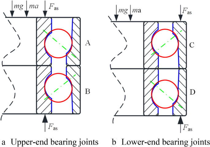

  

  Force diagram of bearing joints under upward acceleration

  According to the force equilibrium in the vertical direction, the normal contact force of each ball in bearings A and D can be obtained as

  $$ \begin{aligned} T_{D \uparrow } & = T_{A \uparrow } = \frac{{F_{as} + {{mg} \mathord{\left/ {\vphantom {{mg} 2}} \right. \kern-\nulldelimiterspace} 2} + {{ma} \mathord{\left/ {\vphantom {{ma} 2}} \right. \kern-\nulldelimiterspace} 2}}}{{n_{b} \sin \alpha_{b} }} \\ {\kern 1pt} & = \frac{{{M \mathord{\left/ {\vphantom {M {\left( {T_{C} \cdot d_{M} } \right)}}} \right. \kern-\nulldelimiterspace} {\left( {T_{C} \cdot d_{M} } \right)}} + {{mg} \mathord{\left/ {\vphantom {{mg} 2}} \right. \kern-\nulldelimiterspace} 2} + {{ma} \mathord{\left/ {\vphantom {{ma} 2}} \right. \kern-\nulldelimiterspace} 2}}}{{n_{b} \sin \alpha_{b} }}, \\ \end{aligned} $$

  (12)

  where n_b is the number of balls in a single bearing, α_b is the contact angle of each ball in the upper- and lower-end bearing joints, d_M is the diameter of the pre-tension nut, and M and T_C are the torque and torque coefficient of the pre-tension nut, respectively.

  The inner and outer rings in a bearing are connected by spring elements distributed around the raceway, which provides the stiffness at both ends to sustain the ball screw. Based on the Hertz contact theory, the relationship between the contact force and the local deformation at the contact point is obtained. The normal contact stiffness of a single ball in bearings A and D can then be derived as

  $$ k_{D \uparrow } = k_{A \uparrow } = \frac{3}{2}K_{h}^{{{2 \mathord{\left/ {\vphantom {2 3}} \right. \kern-\nulldelimiterspace} 3}}} T_{A}^{{{1 \mathord{\left/ {\vphantom {1 3}} \right. \kern-\nulldelimiterspace} 3}}} . $$

  (13)

  Therefore, the equivalent axial stiffness of the upper-end bearing A and lower-end bearing D can be derived as

  $$ \begin{aligned} K_{D \uparrow } \left( a \right) & = K_{A \uparrow } \left( a \right) = \frac{3}{2}K_{h}^{{{2 \mathord{\left/ {\vphantom {2 3}} \right. \kern-\nulldelimiterspace} 3}}} \left( {\frac{M}{{T_{c} \cdot d}} + \frac{m \cdot (a + g)}{2}} \right)^{{{1 \mathord{\left/ {\vphantom {1 3}} \right. \kern-\nulldelimiterspace} 3}}} \\ & \quad \cdot \sin^{{{5 \mathord{\left/ {\vphantom {5 3}} \right. \kern-\nulldelimiterspace} 3}}} \alpha_{b} \cdot \left( {N_{b} \cdot n_{b} } \right)^{{{2 \mathord{\left/ {\vphantom {2 3}} \right. \kern-\nulldelimiterspace} 3}}} \cdot c_{wb} , \\ \end{aligned} $$

  (14)

  where c_wb is the weight coefficient of the equivalent axial stiffness of the bearing joints and has the value of 0.9.

  Based on the principle of deformation compatibility, the normal contact force of each ball in bearing B at the upper end and bearing C at the lower end can be expressed as

  $$ \begin{aligned} T_{C \uparrow } & = T_{B \uparrow } \\ & = \left\{ \begin{aligned} & \frac{{\left( {2\left( {{M \mathord{\left/ {\vphantom {M {\left( {T_{c} \cdot d} \right)}}} \right. \kern-\nulldelimiterspace} {\left( {T_{c} \cdot d} \right)}}} \right)^{{{2 \mathord{\left/ {\vphantom {2 3}} \right. \kern-\nulldelimiterspace} 3}}} - \left( {{M \mathord{\left/ {\vphantom {M {\left( {T_{c} \cdot d} \right)}}} \right. \kern-\nulldelimiterspace} {\left( {T_{c} \cdot d} \right)}} + {{m \cdot (a + g)} \mathord{\left/ {\vphantom {{m \cdot (a + g)} 2}} \right. \kern-\nulldelimiterspace} 2}} \right)^{{{2 \mathord{\left/ {\vphantom {2 3}} \right. \kern-\nulldelimiterspace} 3}}} } \right)^{{{3 \mathord{\left/ {\vphantom {3 2}} \right. \kern-\nulldelimiterspace} 2}}} }}{{n_{b} \sin \alpha_{b} }}, \\ & \quad \left( {\frac{m \cdot a}{2} < 1.83\frac{M}{{T_{c} \cdot d}} - \frac{m \cdot g}{2}} \right), \\ & 0,\quad \left( {\frac{m \cdot a}{2} \ge 1.83\frac{M}{{T_{c} \cdot d}} - \frac{m \cdot g}{2}} \right). \\ \end{aligned} \right. \\ \end{aligned} $$

  (15)

  Similarly, the axial contact stiffness of bearing B at the upper end and bearing C at the lower end can be expressed as

  $$ \begin{aligned} K_{C \uparrow } \left( a \right) & = K_{B \uparrow } \left( a \right) \\ & = \left\{ \begin{aligned} & \frac{3}{2}K_{h}^{{{2 \mathord{\left/ {\vphantom {2 3}} \right. \kern-\nulldelimiterspace} 3}}} \left( {\left( {2\left( {\frac{M}{{T_{c} \cdot d}}} \right)^{{{2 \mathord{\left/ {\vphantom {2 3}} \right. \kern-\nulldelimiterspace} 3}}} - \left( {\frac{M}{{T_{c} \cdot d}} + \frac{m \cdot (a + g)}{2}} \right)^{{{2 \mathord{\left/ {\vphantom {2 3}} \right. \kern-\nulldelimiterspace} 3}}} } \right)^{{{3 \mathord{\left/ {\vphantom {3 2}} \right. \kern-\nulldelimiterspace} 2}}} } \right)^{{{1 \mathord{\left/ {\vphantom {1 3}} \right. \kern-\nulldelimiterspace} 3}}} \\ & \quad \cdot \sin^{{{5 \mathord{\left/ {\vphantom {5 3}} \right. \kern-\nulldelimiterspace} 3}}} \alpha_{b} \cdot \left( {N_{b} \cdot n_{b} } \right)^{{{2 \mathord{\left/ {\vphantom {2 3}} \right. \kern-\nulldelimiterspace} 3}}} \cdot c_{wb} ,{\kern 1pt} \;\left( {\frac{m \cdot (a + g)}{2} < 1.83\frac{M}{{T_{c} \cdot d}}} \right), \\ & 0,\quad \left( {\frac{m \cdot (a + g)}{2} \ge 1.83\frac{M}{{T_{c} \cdot d}}} \right). \\ \end{aligned} \right. \\ \end{aligned} $$

  (16)

  Therefore, when the spindle system accelerates upward, the stiffness of the upper end bearing joints is

  $$ K_{U \uparrow } = \max \left( {K_{A \uparrow } ,K_{B \uparrow } } \right) \cdot c_{wb} . $$

  (17)

  The stiffness of the lower-end bearing joints is

  $$ K_{L \uparrow } = \max (K_{C \uparrow } ,K_{D \uparrow } ) \cdot c_{wb} . $$

  (18)

• (2) Upward deceleration

  Figure 6(a)–(b) show the force analysis of the upper- and lower-end bearing joints under upward deceleration. As shown in Figure 6(a)–(b), during upward deceleration, except for the downward direction of the inertial force, the other forces are the same as those under upward acceleration.

  Figure 6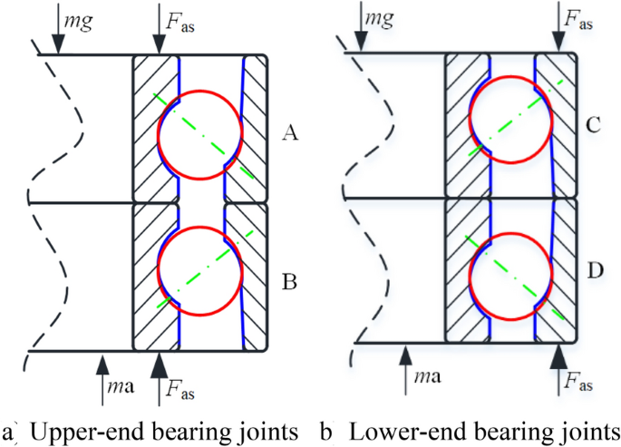

  

  Force diagram of bearing joints under upward deceleration

  According to the force equilibrium of the single bearing in the vertical direction, the normal contact force of each ball in bearings A and D is calculated as

  $$ \begin{aligned} T_{D \downarrow } & = T_{A \downarrow } \\ & = \left\{ \begin{aligned} & \frac{{{M \mathord{\left/ {\vphantom {M {\left( {T_{c} \cdot d} \right)}}} \right. \kern-\nulldelimiterspace} {\left( {T_{c} \cdot d} \right)}} + \left( {m \cdot g} \right)/2 - \left( {m \cdot a} \right)/2}}{{n_{b} \sin \alpha_{b} }},\;\left( {\frac{ma}{2} < \frac{mg}{2}} \right), \\ & \frac{{\left( {2\left( {\left( {{M \mathord{\left/ {\vphantom {M {\left( {T_{c} \cdot d} \right)}}} \right. \kern-\nulldelimiterspace} {\left( {T_{c} \cdot d} \right)}}} \right)} \right)^{{{2 \mathord{\left/ {\vphantom {2 3}} \right. \kern-\nulldelimiterspace} 3}}} - \left( {{M \mathord{\left/ {\vphantom {M {\left( {T_{c} \cdot d} \right)}}} \right. \kern-\nulldelimiterspace} {\left( {T_{c} \cdot d} \right)}} + {{\left( {m \cdot a} \right)} \mathord{\left/ {\vphantom {{\left( {m \cdot a} \right)} 2}} \right. \kern-\nulldelimiterspace} 2} - {{\left( {m \cdot g} \right)} \mathord{\left/ {\vphantom {{\left( {m \cdot g} \right)} 2}} \right. \kern-\nulldelimiterspace} 2}} \right)^{{{2 \mathord{\left/ {\vphantom {2 3}} \right. \kern-\nulldelimiterspace} 3}}} } \right)^{{{3 \mathord{\left/ {\vphantom {3 2}} \right. \kern-\nulldelimiterspace} 2}}} }}{{n_{b} \sin \alpha_{b} }}, \\ {\kern 1pt} & \quad {\kern 1pt} \left( {\frac{mg}{2} \le \frac{ma}{2} \le 1.83\left( {\frac{M}{{T_{c} \cdot d}}} \right) + \frac{mg}{2}} \right), \\ & 0,\quad \left( {\frac{ma}{2} > 1.83\left( {\frac{M}{{T_{c} \cdot d}}} \right) + \frac{mg}{2}} \right). \\ \end{aligned} \right. \\ \end{aligned} $$

  (19)

  Similarly, according to the Hertz contact theory, when the spindle system decelerates upwards with the acceleration magnitude of a, the equivalent axial stiffness for a single ball in bearings A and D can be derived as

  $$ k_{D \downarrow } = k_{A \downarrow } = \frac{3}{2}K_{h}^{{{2 \mathord{\left/ {\vphantom {2 3}} \right. \kern-\nulldelimiterspace} 3}}} T_{A}^{{{1 \mathord{\left/ {\vphantom {1 3}} \right. \kern-\nulldelimiterspace} 3}}} . $$

  (20)

  Therefore, the equivalent axial stiffness for bearings A and D can be derived using

  $$ \begin{aligned} K_{D \downarrow } \left( a \right) & = K_{A \downarrow } \left( a \right) \\ & = \left\{ \begin{aligned} & \frac{3}{2}K_{h}^{{{2 \mathord{\left/ {\vphantom {2 3}} \right. \kern-\nulldelimiterspace} 3}}} \left( {\frac{M}{{T_{c} \cdot d}} + \frac{m \cdot g}{2} - \frac{m \cdot a}{2}} \right)^{{{1 \mathord{\left/ {\vphantom {1 3}} \right. \kern-\nulldelimiterspace} 3}}} \cdot \sin^{{{5 \mathord{\left/ {\vphantom {5 3}} \right. \kern-\nulldelimiterspace} 3}}} \alpha_{b} \cdot \left( {n_{b} } \right)^{{{2 \mathord{\left/ {\vphantom {2 3}} \right. \kern-\nulldelimiterspace} 3}}} \cdot c_{wb} , \\ & \quad \left( {\frac{m \cdot a}{2} < \frac{m \cdot g}{2}} \right), \\ & \frac{3}{2}K_{h}^{{{2 \mathord{\left/ {\vphantom {2 3}} \right. \kern-\nulldelimiterspace} 3}}} \left( {\left( {2\left( {\frac{M}{{T_{c} \cdot d}}{\kern 1pt} } \right)^{{{2 \mathord{\left/ {\vphantom {2 3}} \right. \kern-\nulldelimiterspace} 3}}} - \left( {\frac{M}{{T_{c} \cdot d}} + \frac{m \cdot a}{2} - \frac{m \cdot g}{2}} \right)^{{{2 \mathord{\left/ {\vphantom {2 3}} \right. \kern-\nulldelimiterspace} 3}}} } \right)^{{{3 \mathord{\left/ {\vphantom {3 2}} \right. \kern-\nulldelimiterspace} 2}}} } \right)^{{{1 \mathord{\left/ {\vphantom {1 3}} \right. \kern-\nulldelimiterspace} 3}}} \\ & \quad \cdot \sin^{{{5 \mathord{\left/ {\vphantom {5 3}} \right. \kern-\nulldelimiterspace} 3}}} \alpha_{b} \cdot \left( {n_{b} } \right)^{{{2 \mathord{\left/ {\vphantom {2 3}} \right. \kern-\nulldelimiterspace} 3}}} \cdot c_{wb} ,{\kern 1pt} \\ {\kern 1pt} & \quad \left( {\frac{m \cdot g}{2} \le \frac{m \cdot a}{2} \le 1.83\left( {\frac{M}{{T_{c} \cdot d}}} \right) + \frac{m \cdot g}{2}} \right), \\ & 0,\quad \left( {\frac{m \cdot a}{2} > 1.83\left( {\frac{M}{{T_{c} \cdot d}}} \right) + \frac{m \cdot g}{2}} \right). \\ \end{aligned} \right. \\ \end{aligned} $$

  (21)

  Similarly, according to the theory of deformation compatibility, the normal contact force of a single ball in bearing C and bearing B is

  $$ \begin{aligned} T_{C \downarrow } & = T_{B \downarrow } \\ & = \left\{ \begin{array} {*{20}ll} \frac{{\left( {2\left( {{M \mathord{\left/ {\vphantom {M {\left( {T_{c} \cdot d} \right)}}} \right. \kern-\nulldelimiterspace} {\left( {T_{c} \cdot d} \right)}}} \right)^{{{2 \mathord{\left/ {\vphantom {2 3}} \right. \kern-\nulldelimiterspace} 3}}} - \left( {{M \mathord{\left/ {\vphantom {M {\left( {T_{c} \cdot d} \right)}}} \right. \kern-\nulldelimiterspace} {\left( {T_{c} \cdot d} \right)}} + \left( {m \cdot g} \right)/2 - \left( {m \cdot a} \right)/2} \right)^{{{2 \mathord{\left/ {\vphantom {2 3}} \right. \kern-\nulldelimiterspace} 3}}} } \right)^{{{3 \mathord{\left/ {\vphantom {3 2}} \right. \kern-\nulldelimiterspace} 2}}} }}{{n_{b} \sin \alpha_{b} }}, & \left( {\frac{ma}{2} < \frac{mg}{2}} \right), \\ \frac{{{M \mathord{\left/ {\vphantom {M {\left( {T_{c} \cdot d} \right)}}} \right. \kern-\nulldelimiterspace} {\left( {T_{c} \cdot d} \right)}} + {{\left( {m \cdot a} \right)} \mathord{\left/ {\vphantom {{\left( {m \cdot a} \right)} 2}} \right. \kern-\nulldelimiterspace} 2} - {{\left( {m \cdot g} \right)} \mathord{\left/ {\vphantom {{\left( {m \cdot g} \right)} 2}} \right. \kern-\nulldelimiterspace} 2}}}{{n_{b} \sin \alpha_{b} }}{\kern 1pt}, & \left( {\frac{ma}{2} \ge \frac{mg}{2}} \right). \\ \end{array} \right. \\ \end{aligned} $$

  (22)

  The axial contact stiffness of bearing B and bearing C is expressed as

  $$ \begin{aligned} K_{C \downarrow } \left( a \right) & = K_{B \downarrow } \left( a \right) \\ & = \left\{ \begin{aligned} & \frac{3}{2}K_{h}^{{{2 \mathord{\left/ {\vphantom {2 3}} \right. \kern-\nulldelimiterspace} 3}}} \left( {\left( {2\left( {\frac{M}{{T_{c} \cdot d}}} \right)^{{{2 \mathord{\left/ {\vphantom {2 3}} \right. \kern-\nulldelimiterspace} 3}}} - \left( {\frac{M}{{T_{c} \cdot d}} + \frac{m \cdot g}{2} - \frac{m \cdot a}{2}} \right)^{{{2 \mathord{\left/ {\vphantom {2 3}} \right. \kern-\nulldelimiterspace} 3}}} } \right)^{{{3 \mathord{\left/ {\vphantom {3 2}} \right. \kern-\nulldelimiterspace} 2}}} } \right)^{{{1 \mathord{\left/ {\vphantom {1 3}} \right. \kern-\nulldelimiterspace} 3}}} \\ & \quad \cdot \sin^{{{5 \mathord{\left/ {\vphantom {5 3}} \right. \kern-\nulldelimiterspace} 3}}} \alpha_{b} \cdot \left( {N_{b} \cdot n_{b} } \right)^{{{2 \mathord{\left/ {\vphantom {2 3}} \right. \kern-\nulldelimiterspace} 3}}} \cdot c_{wb} , \quad \left( {\frac{ma}{2} < \frac{mg}{2}} \right), \\ & \frac{3}{2}K_{h}^{{{2 \mathord{\left/ {\vphantom {2 3}} \right. \kern-\nulldelimiterspace} 3}}} \left( {\frac{M}{{T_{c} \cdot d}} + \frac{m \cdot a}{2} - \frac{m \cdot g}{2}} \right)^{{{1 \mathord{\left/ {\vphantom {1 3}} \right. \kern-\nulldelimiterspace} 3}}} \\ & \quad \cdot \sin^{{{5 \mathord{\left/ {\vphantom {5 3}} \right. \kern-\nulldelimiterspace} 3}}} \alpha_{b} \cdot \left( {N_{b} \cdot n_{b} } \right)^{{{2 \mathord{\left/ {\vphantom {2 3}} \right. \kern-\nulldelimiterspace} 3}}} \cdot c_{wb} ,\quad \left( {\frac{ma}{2} \ge \frac{mg}{2}} \right). \\ \end{aligned} \right. \\ \end{aligned} $$

  (23)

  Therefore, when the spindle system decelerates upwards, the stiffness of the upper-end bearing joints is

  $$ K_{U \downarrow } = \max (K_{A \downarrow } ,K_{B \downarrow } ) \cdot c_{wb} . $$

  (24)

  The stiffness of the lower-end bearing joints is

  $$ K_{L \downarrow } = \max \left( {K_{C \downarrow } ,K_{D \downarrow } } \right) \cdot c_{wb} . $$

  (25)

2.3.3 Calculation of Axial Stiffness of the Ball Screw

In the axial fixed-fixed support mode, the lead screw is divided into two sections by screw-nut joints. The servo motor drives the rotation of the screw shaft, causing the upper section of the screw shaft to rotate. In addition, the upper and lower sections of the screw shaft are axially restrained by the bearings. However, the lengths of the upper and lower sections of the screw shaft change as the spindle system moves up and down. As a result, the axial tensile/compressive stiffness of the upper and lower sections and the axial torsional stiffness of the upper section of the screw shaft change. The expressions for the stiffness of the upper and lower sections of the screw shaft can be obtained as

$$ K_{us1} (z) = \frac{{4GE\uppi ^{3} d_{1}^{4} }}{{16G\uppi ^{2} d_{1}^{2} \left( {L - z} \right) + 32p^{2} E\left( {L - z} \right)}}, $$

(26)

$$ K_{ds1} (z) = \frac{{\uppi d_{1}^{2} E}}{4z}, $$

(27)

where $K_{us1}$ is the axial stiffness of the upper section of the screw shaft, $K_{ds1}$ is the axial stiffness of the lower section of the screw shaft, d₁ is the bottom diameter of the screw shaft, E is the elastic modulus, G is the shear modulus, and p is the screw pitch.

2.3.4 Calculation of Transmission Stiffness

The transmission stiffness in the transmission direction consists of the axial stiffness of both the upper and lower sections of the screw shaft and the equivalent axial stiffness of the screw-nut joints and bearing joints, as shown in Figure 2.

Therefore, the transmission stiffness under upward acceleration in the transmission direction can be calculated as

$$ \begin{aligned} k_{e \uparrow } \left( {a,z} \right) & = \\ & \quad \frac{{\left( {\frac{{K_{us} (z) \cdot K_{U \uparrow } (a)}}{{K_{us} (z) + K_{U \uparrow } (a)}} + \frac{{K_{ds} (z) \cdot K_{L \uparrow } (a)}}{{K_{ds} (z) + K_{L \uparrow } (a)}}} \right) \cdot K_{nut \uparrow } \left( a \right)}}{{\left( {\frac{{K_{us} (z) \cdot K_{U \uparrow } (a)}}{{K_{us} (z) + K_{U \uparrow } (a)}} + \frac{{K_{ds} (z) \cdot K_{L \uparrow } (a)}}{{K_{ds} (z) + K_{L \uparrow } (a)}}} \right) + K_{nut \uparrow } \left( a \right)}}. \\ \end{aligned} $$

(28)

Similarly, the transmission stiffness under upward deceleration in the transmission direction can be calculated as

$$ \begin{aligned} k_{e \downarrow } (a,z) & = \\ & \quad \frac{{\left( {\frac{{K_{us} (z) \cdot K_{U \downarrow } (a)}}{{K_{us} (z) + K_{U \downarrow } (a)}} + \frac{{K_{ds} (z) \cdot K_{L \downarrow } (a)}}{{K_{ds} (z) + K_{L \downarrow } (a)}}} \right) \cdot K_{nut \downarrow } (a)}}{{\left( {\frac{{K_{us} (z) \cdot K_{U \downarrow } (a)}}{{K_{us} (z) + K_{U \downarrow } (a)}} + \frac{{K_{ds} (z) \cdot K_{L \downarrow } (a)}}{{K_{ds} (z) + K_{L \downarrow } (a)}}} \right) + K_{nut \downarrow } (a)}}. \\ \end{aligned} $$

(29)

3 Experimental Verification

3.1 Experimental Configuration

The vertical ball screw feed system in a miniature vertical machining center without counterweight was used for dynamic testing, as shown in Figure 7. Its parameter values are shown in Table 1. The spindle system was mounted on the bed with a pair of linear guides (grooves with four semicircular arcs) and driven by a screw with a 45 mm diameter and 16 mm pitch. The rated dynamic load P_d was 31.15 kN. The initial preload of the screw-nut joint was set to 0.1P_d, and both ends of the screw shaft were supported by angular contact ball bearings (30 TAC 62 B, NSK). The displacement of the spindle system in the Z direction under upward acceleration and deceleration was measured using a laser interferometer (XL-80, Renishaw), as shown in Figure 1. The measuring mirror was mounted on the downside in front of the spindle box, and the reflector was mounted on the worktable parallel to the lower plane of the spindle box. The sampling frequency was 50 kHz. During testing, the spindle system moved up and down along the Z-axis around the bottom end of the screw (z/L = 0.9) under different accelerations and decelerations. A maximum feed rate of 0.1333 m/s was set because it was large enough to generate a segment of constant acceleration. The acceleration values in the constant acceleration segment were changed by modifying the time constant and the agility time constant.

Figure 7

Experimental setup for characterizing the vibrations of the vertical feed system

Table 1 Simulation parameters

Owing to the limitations of the machine tool, the maximum acceleration could not exceed 1g. The time constant and agility time constant could only be integers determined by the settings of the CNC system. Simultaneously, the functional relationship between the acceleration and the two parameters should be satisfied. Only the acceleration values of 0.1g, 0.2g, 0.28g, 0.42g, 0.55g, and 0.8g satisfy the above relationship. The vibration characteristics under these acceleration values were obtained. In this work, the three representative acceleration values selected for analysis were 0.2g, 0.55g, and 0.8g. The corresponding constant acceleration durations were 0.064, 0.018, and 0.008 s, respectively. Figure 8 shows the acceleration and deceleration curves output by the feed system when the constant acceleration in the segment of constant acceleration was 0.2g. Similar acceleration and deceleration curves were obtained at the other constant acceleration values.

Figure 8

S type acceleration and deceleration process

3.2 Experimental Vibration Characteristics

From Figure 8, it can be seen that the two segments t1t2 and t3t4 were upward acceleration and deceleration sections, respectively. The upward acceleration and deceleration are transient variables. To obtain the vibration frequency under a certain acceleration, the power spectral density (PSD) can be used. The PSD method is similar to the frequency response function, both of which can be used to represent the vibration spectrum in the transmission direction. In this study, the maximum entropy spectral estimation, which is a parameterized model spectral estimation method also known as Burg’s method [31], was used, and the PSD of the system, which was on the order of 500, was obtained. The number of execution points was 131072. The vibration frequencies in the transmission direction were mainly found within the first-order frequency range. The results are shown in Figure 9. It can be seen that the vibration frequencies varied under different accelerations.

Figure 9

Frequency response of spindle system under different accelerations and decelerations

For comparison, the natural frequencies under different upward accelerations and decelerations are summarized in Table 2. As the acceleration of the spindle system in the upwards direction increased from 0.2g to 0.8g, the natural frequency decreased by 3%. As the spindle system deceleration in the upward direction increased from 0.2g to 0.8g, the natural frequency decreased by 5.6%. When the acceleration value reached 0.8 g, the difference between the natural frequencies for upward acceleration and deceleration was 14.9%. The results clearly show that the direction and magnitude of the acceleration can cause the spindle system to exhibit varying degrees of vibration in the transmission direction.

Table 2 Comparison of the experimental and theoretical natural frequency values of the system

4 Results and Discussion

4.1 Comparison of Theoretical and Experimental Results

To verify the theoretical model, the simulation curves under the conditions of z/L = 0.9, F_as = 35 kN, and P_d = 31.15 kN were compared with the experimental results for the acceleration magnitudes of 2 m/s², 5.5 m/s² and 8 m/s². The results are shown in Table 2.

As can be clearly seen in Table 2, the predictions of the variable-coefficient lumped parameter model are consistent with the experimental vibration results. Regardless of the direction and magnitude of the acceleration, the differences between the predicted and experimental frequency values are less than 10%. Therefore, the analytical model presented in this study can accurately reflect the dynamic characteristics of the vertical ball screw feed system.

4.2 Simulation Results

Simulation analysis was performed to investigate the variation of the natural frequency. The spindle system was first located at the position z/L = 0.9. The rated dynamic load was set to 31.15 kN and screw tension force to 35 kN. The other parameters were kept constant and one of the above three parameters was varied to determine its effects on the natural frequency of the system. The results for the influence of these parameters on the natural frequency under acceleration and deceleration are shown in Figure 10. The figure shows the influence of eight combinations of the three parameters and acceleration direction on the variation of the natural frequency with the acceleration magnitude. The symbols in the legend in Figure 10 correspond to the eight combinations of parameter values and states listed in Table 3.

Figure 10

Comparison of natural frequency under acceleration and deceleration as a function of P_d, F_as, z/L

Table 3 Symbols for the eight combinations of parameter values and states

From Figure 10, it can be seen that varying the spindle system position, screw-tension force, and rated dynamic load of the screw-nut joints does not change the trends of the natural frequency under acceleration and deceleration. Consequently, the natural frequencies under acceleration and deceleration are always different. This is because when the spindle system accelerates upward, the direction of the inertial force is downward. However, when the spindle system decelerates upward, the direction of the inertial force is upward. In addition, the inertial force increases with an increase in the acceleration. As a result, the forces acting on the joints are different under acceleration and deceleration, which leads to a difference in the transmission stiffness and ultimately, a difference in the natural frequency.

Meanwhile, regardless of how the parameters change, the maximum percentage difference between the natural frequencies under acceleration and deceleration always occurs at 1g. This is closely related to the stiffness of the screw-nut joints. The stiffness of nut A is greater than that of nut B before the value of 1g. At this time, the stiffness of the screw-nut joints is determined by the stiffness of nut A. However, the stiffness of nut B is greater than that of nut A after the value of 1g. The stiffness of the screw-nut joints is determined by the stiffness of nut B. When the acceleration value is 1g, the stiffness of nut A is equal to the stiffness of nut B. The stiffness of the screw-nut joints is then equal to both stiffnesses and has the smallest value at this time. However, the stiffness of the screw-nut joints changes the overall variation in the natural frequency as well as the maximum percentage discrepancy of the natural frequency under upward acceleration and deceleration.

It is of interest to study the differences in the impact of the rated dynamic load (F_a), screw-tension force (F_as), and the spindle system position (z/L) on the overall variation and the maximum percentage discrepancy of the natural frequency. The overall variation (δ) and the maximum percentage discrepancy (β) in the predicted natural frequencies were calculated as

$$ \delta_{e} = \frac{{\left( {\omega_{ie} - \omega_{je} } \right)}}{{\omega_{ie} }} \times 100\% , $$

(30)

$$ \beta = \frac{{\left( {\omega_{ka} - \omega_{la} } \right)}}{{\omega_{la} }} \times 100\% , $$

(31)

where w_ie and w_je are the maximum and minimum natural frequency. The subscripts e = 1 and e = 2 represent upward acceleration and downward acceleration respectively, while w_ka and w_la represents the natural frequency at 1g under acceleration and deceleration, respectively.

Figure 11 shows the overall variation of the natural frequency and the maximum percentage difference as functions of the rated dynamic load, screw-tension force, and spindle system position. The rated dynamic load of the screw-nut joint was set to 32 kN, 42 kN, 52 kN, 62 kN, 72 kN, 82 kN, and 92 kN; the screw-tension force was set to 35 kN, 45 kN, 55 kN, 65 kN, and 75 kN; and the spindle system position (z/L) was set to 0.1, 0.2, 0.3, 0.4, 0.5, 0.6, 0.7, 0.8, and 0.9. The values for the other important parameters of the ball screw feed system remained unchanged in the simulation.

Figure 11

Variation and difference of the natural frequency under the effect of different parameters

From Figure 11(a), it can be observed that as the rated dynamic load increases, the overall variation and the maximum percentage difference of the natural frequency increase. Conversely, as shown in Figure 11(b), as the screw tension force increases, the overall variation and the maximum percentage difference decrease. However, as shown in Figure 11(c), as the position of the spindle system changes from the top to the bottom, the overall variation and the maximum percentage difference first decrease and then increase. Combining Figure 11(a)–(c) and Table 4, it can be seen that the rated dynamic load has the greatest impact, the spindle system position has a relatively light impact, and the impact of the screw-tension force is not as clear.

Table 4 Comparison of overall variation (δ) and maximum percentage discrepancy (β)

5 Conclusions

A variable-coefficient lumped parameter dynamic model of a vertical ball screw feed system without counterweight that considers the influence of the spindle system weight and the inertial force under acceleration and deceleration on the kinematic joint stiffness was presented. Simulations and experiments were performed on a ball screw feed system without counterweight to study the differences in the natural frequency of the system under acceleration and deceleration. The influence of the screw tension force, the rated dynamic load of the screw-nut joints, and the position of the spindle system on its natural frequency was also analyzed. The main conclusions are as follows.

• (1) The natural frequency of the feed system increases when the spindle system accelerates upwards. The natural frequency first decreases and then increases when the spindle system decelerates upwards. The maximum difference of the natural frequencies between upward acceleration and deceleration is significant and can reach as high as 15.4%.

• (2) Compared with the screw-tension force, the rated dynamic load of screw-nut joints and the spindle system position play a major role in determining the natural frequency of the feed system under upward acceleration and deceleration.

• (3) When designing a vertical ball screw feed system without counterweight and optimizing the system vibration control algorithms for high-quality machining, the variation in the natural frequency under acceleration and deceleration needs to be considered. To obtain relatively stable dynamic characteristics for a system with a fixed support mode at both ends, the machine tool should ideally be run in the middle position in the entire stroke during high-quality machining.

References

X Li, J Zhang, W Zhao, et al. A zero phase error tracking based path precompensation method for high-speed machining. Proceedings of the Institution of Mechanical Engineers, Part C: Journal of Mechanical Engineering Science, 2016, 230: 230-239.
X Yang, D Lu, J Zhang, et al. Dynamic electromechanical coupling resulting from the air-gap fluctuation of the linear motor in machine tools. International Journal of Machine Tools and Manufacture, 2015, 94: 100-108.
H Shi, D Zhang, J Yang, et al. Experiment-based thermal error modeling method for dual ball screw feed system of precision machine tool. The International Journal of Advanced Manufacturing Technology, 2016, 82: 1693-1705.
F Y Pai, T M Yeh, Y H Hung. Analysis on accuracy of bias, linearity and stability of measurement system in ball screw processes by simulation. Sustainability, 2015, 7(11):15464-15486.
C Zhang, Y Chen. Tracking control of ball screw drives using ADRC and equivalent-error-model-based feedforward control. IEEE Transactions on Industrial Electronics, 2016, 63(12): 7682-7692.
X Gao, B Li, J Hong, et al. Stiffness modeling of machine tools based on machining space analysis. International Journal of Advanced Manufacturing Technology, 2016, 86: 1-14.
D Lu, Q Liu, H Liu, et al. Dynamic error of CNC machine tools: a state-of-the-art review. International Journal of Advanced Manufacturing Technology, 2020, 106: 1869-1891.
J P Hung, Y L Lai, T L Luo, et al. Analysis of the machining stability of a milling machine considering the effect of machine frame structure and spindle bearings: experimental and finite element approaches. The International Journal of Advanced Manufacturing Technology, 2013, 68(9): 2393-2405.
Z Pandilov, A Milecki, A Nowak, et al. Virtual modeling and simulation of a CNC machine feed drive system. Annals of the Faculty of Engineering, 2016, 39(4): 37-54.
R Wang, T Zhao, P Ye, et al. Three-dimensional modeling for predicting the vibration modes of twin ball screw driving table. Chinese Journal of Mechanical Engineering, 2014, 27(1): 211-218.
J M Zhu, T C Zhang, X Li. Dynamic characteristic analysis of ball screw feed system based on stiffness characteristic of mechanical joints. Journal of Mechanical Engineering, 2015, 51(17): 72-82. (in Chinese)
H Liu, D Lu, J Zhang, et al. Receptance coupling of multi-subsystem connected via a wedge mechanism with application in the position-dependent dynamics of ballscrew drives. Journal of Sound and Vibration, 2016, 376: 166-181.
H J Zhang, H Liu, C Du, et al. Dynamics analysis of a slender ball-screw feed system considering the changes of the worktable position. Proceedings of the Institution of Mechanical Engineers, Part C: Journal of Mechanical Engineering Science, 2019, 233(8): 2685-2695.
M Silva, O Brüls, J Swevers, et al. Computer-aided integrated design for machines with varying dynamics. Mechanism and Machine Theory, 2009, 44: 1733-1745.
B Paijmans, W Symens, H V Brussel, et al. Experimental identification of interpolating affine LPV models for mechatronic systems with one varying parameter. European Journal of Control, 2008, 14: 16-29.
M Hanifzadegan, R Nagamune. Tracking and structural vibration control of flexible ball–screw drives with dynamic variations. IEEE/ASME Transactions on Mechatronics, 2015, 20(1): 133-142.
M Wang, T Zan, X Gao, et al. Suppression of the time-varying vibration of ball screws induced from the continuous movement of the nut using multiple tuned mass dampers. International Journal of Machine Tools & Manufacture, 2016: 41-49.
H Liu, J Zhang, W Zhao. An intelligent non-collocated control strategy for ball-screw feed drives with dynamic variations. Engineering, 2017, 3(5): 641-647.
A Verl, S Frey. Correlation between feed velocity and preloading in ball screw drives. CIRP Annals, 2010, 59(1): 429-432
B Li, B Luo, X Mao, et al. A new approach to identifying the dynamic behavior of CNC machine tools with respect to different worktable feed speeds. International Journal of Machine Tools and Manufacture, 2013, 72: 73-84.
H J Zhang, J Zhang, H Liu, et al. Dynamic modeling and analysis of the high-speed ball screw feed system. Proceedings of the Institution of Mechanical Engineers, Part B: Journal of Engineering Manufacture, 2015, 229(5): 870-877.
X Mao, Q Liu, B Li, et al. Investigation on the dynamic behavior of machine tool with respect to different worktable feed rates. 2016 7th International Conference on Mechanical and Aerospace Engineering (ICMAE), IEEE, 2016: 253-256.
J S Chen, Y K Huang, C C Cheng. Mechanical model and contouring analysis of high-speed ball-screw drive systems with compliance effect. The International Journal of Advanced Manufacturing Technology, 2004, 24(3-4): 241-250.
J Zhang, H Zhang, C Du, et al. Research on the dynamics of ball screw feed system with high acceleration. International Journal of Machine Tools and Manufacture, 2016, 111: 9-16.
M Law, A S Phani, Y Altintas, et al. Position-dependent multibody dynamic modeling of machine tools based on improved reduced order models. Journal of Manufacturing Science and Engineering, 2013, 135: 2-11.
M Law, Y Altintas, A S Phani. Rapid evaluation and optimization of machine tools with position dependent stability. International Journal of Machine Tools and Manufacture, 2013, 68: 81-90.
M Law, S Ihlenfeldt. A frequency-based substructuring approach to efficiently model position-dependent dynamics in machine tools. Proceedings of the Institution of Mechanical Engineers, Part K: Journal of Multi-body Dynamics, 2015, 229(3): 304-317.
C F Zou, H J Zhang, D Lu, et al. Effect of the screw–nut joint stiffness on the position-dependent dynamics of a vertical ball screw feed system without counterweight. Proceedings of the Institution of Mechanical Engineers, Part C: Journal of Mechanical Engineering Science, 2018, 232(15): 2599-2609.
J Brändlein, P Eschmann, L Hasbargen, et al. Ball and roller bearings: theory, design, and application. 3rd ed. Oxford: John Wiley&Sons, Ltd., 1999.
T A Harris, M N Kotzalas. Advanced concepts of bearing technology: rolling bearing analysis. Boca Raton: CRC Press, 2006.
S M Kay. Modern spectral estimation: Theory and application. PrenticeHall, EnglewoodCliffs, NJ, 1999.
Acknowledgements
The authors sincerely thank Wenming Wei and Lei Wang for his critical discussion and reading during manuscript preparation.
Funding
Supported by Key Program of National Natural Science Foundation of China (Grant No. 51235009) and National Natural Science Foundation of China (Grant No. 51605374).
Author information
Authors and Affiliations
Contributions
CZ carried out the experiment studies and drafted the manuscript. HZ carried out the sequence alignment and revision of the manuscript. All authors read and approved the final manuscript.
Authors’ Information
Cunfan Zou, born in 1983, is currently a PhD candidate at State Key Laboratory for Manufacturing Systems Engineering, Xi’an Jiaotong University, China. Her research interests include mechanical dynamics of high speed precision machine tools.
Huijie Zhang, born in 1983, is currently an engineer at State Key Laboratory for Manufacturing Systems Engineering, Xi’an Jiaotong University, China. He received his PhD degree from Xi’an Jiaotong University, China, in 2014. His research interests include mechanical dynamics of high speed precision machine tools.
Jun Zhang, born in 1978, is currently a professor and a PhD candidate supervisor at State Key Laboratory for Manufacturing Systems Engineering, Xi’an Jiaotong University, China. His research interests include prediction of equipment accuracy driven by large data and high speed machining technology.
Dongdong Song, born in 1984, is currently a PhD candidate at State Key Laboratory for Manufacturing Systems Engineering, Xi’an Jiaotong University, China. His research interests include dynamics and dynamic performance prediction of machine tools and twin-tool machining technology.
Hui Liu, born in1974, is currently an engineer at State Key Laboratory for Manufacturing Systems Engineering, Xi’an Jiaotong University, China. His research interests include dynamics and control of machine tools.
Wanhua Zhao, born in 1965, is currently a professor and a PhD candidate supervisor at State Key Laboratory for Manufacturing Systems Engineering, Xi’an Jiaotong University, China. His research interests include intelligent equipment theory and method based on deep learning.
Corresponding author
Ethics declarations
Competing Interests
The authors declare no competing financial interests.
Rights and permissions
Open Access This article is licensed under a Creative Commons Attribution 4.0 International License, which permits use, sharing, adaptation, distribution and reproduction in any medium or format, as long as you give appropriate credit to the original author(s) and the source, provide a link to the Creative Commons licence, and indicate if changes were made. The images or other third party material in this article are included in the article's Creative Commons licence, unless indicated otherwise in a credit line to the material. If material is not included in the article's Creative Commons licence and your intended use is not permitted by statutory regulation or exceeds the permitted use, you will need to obtain permission directly from the copyright holder. To view a copy of this licence, visit http://creativecommons.org/licenses/by/4.0/.
About this article
Cite this article
Zou, C., Zhang, H., Zhang, J. et al. Acceleration-Dependent Analysis of Vertical Ball Screw Feed System without Counterweight. Chin. J. Mech. Eng. 34, 65 (2021). https://doi.org/10.1186/s10033-021-00575-2
Received:
Revised:
Accepted:
Published:
DOI: https://doi.org/10.1186/s10033-021-00575-2