Optimal Design for Anti-Skid Control of Electric Vehicles by Fuzzy Approach

Abstract

In this paper, a new fuzzy approach is applied to optimal design of the anti-skid control for electric vehicles. The anti-skid control is used to maintain the wheel speed when there are uncertainties. The control is able to provide an appropriate torque for wheels when the vehicle is about to skid. The friction coefficient and the moments of inertia of wheels and motor are considered as uncertain parameters. These nonlinear, bounded and time-varying uncertainties are described by fuzzy set theory. The control is deterministic and is not based on IF-THEN fuzzy rules. Then, the optimal design for this fuzzy system and control cost is proposed by fuzzy information. In this way, the uniform boundedness and uniform ultimate boundedness are guaranteed and the average fuzzy performance is minimized. Numerical simulations show that the control can prevent vehicle skidding with the minimum control cost under uncertainties.

1 Introduction

With people’s consciousness on the environment and the development of motor and battery technology, electric vehicles (EVs) are getting great attention these years [1]. The anti-skid control which is related to the safety is one of focuses in EVs research field. In Ref. [2], a fast feedback control with motor was applied for anti skid control. The braking distance was reduced by 20%. In Ref. [3], an anti-skid controller with PI regulator is designed based on back-EMF observer and dynamic model error observer. The more effective control approach should be available with the fast torque response and accurate feedback of the motors in EVs.

However, the anti skid system includes nonlinearity and uncertainties from motor, wheel and road. These parameters can not be measured precisely such as the friction coefficient. Thus, a fuzzy approach is applied to describing this system in this paper.

Many researches about EV anti skid control have been explored. Most paper use the parameter slip ratio to design control. In Ref. [4], the sliding-mode-observer-based adaptive sliding mode control was presented for EVs. In Ref. [5], the yaw-rate control is proposed based on the slip ratio. In Ref. [6], the parameter slip ratio was used to design a sliding mode control for EVs. Then, a reference slip related to road condition is needed [7, 8]. These approaches are useful. However, more precise control may not be achieved based on slip ratio. In Ref. [9], a road condition estimation approach is proposed. This approach is based on the driving force observer, which is difficult to be applied to engine vehicle. In Ref. [10], a PI controller is proposed without speed sensor. It can reduce the speed detector device and decrease the cost. But, the robustness may be not good enough based on PI control. In Ref. [11], a sliding mode control is applied to anti skid system of EVs. This control can overcome uncertainties.

Uncertainty is inevitable in a practical system. The probability theory is the most widely used method to give a mathematical description of uncertainty and many great achievements are made based on that [12, 13]. However, it may not always be suitable to deal with uncertainty by using the frequency of occurrence [14]. In 1965, Zadeh introduced the fuzzy set theory to describe uncertainty by employing the degree of occurrence [15]. Recently, this theory has been developed and applied to many fields, such as fuzzy choice [16], fuzzy difference equation [17]. By contrast, there are not many explorations between fuzzy set theory and system theory. In this paper, the fuzzy dynamical system is established and the uncertainty in the system is described by fuzzy set theory which is different from the popular T-S fuzzy model or IF-THEN model [18, 19]. These two fuzzy models have been applied to many fields. In Ref. [20], the model was used to design tracking control for nonlinear dynamic systems. In Ref. [21], the time delay problem was taken into consideration. In Ref. [22], a guaranteed cost control method for nonlinear systems was proposed based on Takagi-Sugeno (T-S) fuzzy models. According to the fuzzy dynamical system based on the fuzzy set theory, the optimal design of control is solved for this fuzzy dynamical system when there are multiple tunable parameters. In Ref. [23], the fundamental frame of the fuzzy dynamical system was established. In Ref. [24], the theory was applied to the flexible joint manipulators. In Ref. [25], a fuzzy approach for optimal robust control design of an automotive electronic throttle system was proposed. However, only one parameter was considered in the optimization problem of the previous works. The originality of the paper can be summarized as follows: describing the uncertainties of the EV system by fuzzy set theory; designing a novel high-order robust control; investigating the relationships among the control parameters, system performance, and control cost.

The main contributions are threefold. First, the fuzzy anti-skid dynamical system of EVs is established. The uncertainties and disturbances are taken into consideration based on fuzzy set theory. Second, a novel higher-order control is proposed. It is deterministic and not based on IF-THEN fuzzy rule. By applying this control, we prove that the system is uniformly bounded and uniformly ultimately bounded via the Lyapunov theory [26]. Third, an index combined average fuzzy system performance and control cost is proposed with multiple parameters. By minimizing the index, the optimal design problem is solved.

2 Fuzzy Dynamical Systems with Uncertainties

Before giving the fuzzy dynamical systems, some preliminary knowledges related to fuzzy sets theory are given as follows.

Fuzzy Number. Let ${\mathfrak {S}}$ be a fuzzy set in $\mathbf{R }$, the real number. ${\mathfrak {S}}$ is called fuzzy number if: (i) ${\mathfrak {S}}$ is normal, (ii) ${\mathfrak {S}}$ is convex, (iii) the support of ${\mathfrak {S}}$ is bounded, and (iv) all $\alpha$-cuts are closed intervals in $\mathbf{R }$. In addition, the universe of discourse of a fuzzy number is considered to be its 0-cut.

Fuzzy Arithmetic. Let ${\mathfrak {S}}$ and ${\mathfrak {T}}$ to be two fuzzy numbers and ${\mathfrak {S}}_{\alpha }=[{\mathfrak {s}}_{\alpha }^{-},{\mathfrak {s}}_{\alpha }^{+}]$, ${\mathfrak {T}}_{\alpha }=[{\mathfrak {t}}_{\alpha }^{-},{\mathfrak {t}}_{\alpha }^{+}]$ be their $\alpha$-cuts, $\alpha \in [0,1]$. The addition, subtraction, multiplication, and division of ${\mathfrak {S}}$ and ${\mathfrak {T}}$ are defined as follows,

$$({\mathfrak {S}}+{\mathfrak {T}})_{\alpha }= [{\mathfrak {s}}_{\alpha }^{-}+{\mathfrak {t}}_{\alpha }^{-},{\mathfrak {s}}_{\alpha }^{+}+{\mathfrak {t}}_{\alpha }^{+}],$$

(1)

$$({\mathfrak {S}}-{\mathfrak {T}})_{\alpha }=[\text {min}({\mathfrak {s}}_{\alpha }^{-}-{\mathfrak {t}}_{\alpha }^{-},{\mathfrak {s}}_{\alpha }^{+}-{\mathfrak {t}}_{\alpha }^{+}),\text {max}({\mathfrak {s}}_{\alpha }^{-}-{\mathfrak {t}}_{\alpha }^{-},{\mathfrak {s}}_{\alpha }^{+}-{\mathfrak {t}}_{\alpha }^{+})],$$

(2)

$$\begin{aligned} ({\mathfrak {S}}\cdot {\mathfrak {T}})_{\alpha }& = [\text {min}({\mathfrak {s}}_{\alpha }^{-}{\mathfrak {t}}_{\alpha }^{-},{\mathfrak {s}}_{\alpha }^{-}{\mathfrak {t}}_{\alpha }^{+},{\mathfrak {s}}_{\alpha }^{+}{\mathfrak {t}}_{\alpha }^{-},{\mathfrak {s}}_{\alpha }^{+}{\mathfrak {t}}_{\alpha }^{+}),\nonumber \\& \quad\text {max}({\mathfrak {s}}_{\alpha }^{-}{\mathfrak {t}}_{\alpha }^{-},{\mathfrak {s}}_{\alpha }^{-}{\mathfrak {t}}_{\alpha }^{+},{\mathfrak {s}}_{\alpha }^{+}{\mathfrak {t}}_{\alpha }^{-},{\mathfrak {s}}_{\alpha }^{+}{\mathfrak {t}}_{\alpha }^{+})], \end{aligned}$$

(3)

$$\begin{aligned} ({\mathfrak {S}}/{\mathfrak {T}})_{\alpha } &= [\text {min}({\mathfrak {s}}_{\alpha }^{-}/{\mathfrak {t}}_{\alpha }^{-},{\mathfrak {s}}_{\alpha }^{-}/{\mathfrak {t}}_{\alpha }^{+},{\mathfrak {s}}_{\alpha }^{+}/{\mathfrak {t}}_{\alpha }^{-},{\mathfrak {s}}_{\alpha }^{+}/{\mathfrak {t}}_{\alpha }^{+}),\nonumber \\& \quad \text {max}({\mathfrak {s}}_{\alpha }^{-}/{\mathfrak {t}}_{\alpha }^{-},{\mathfrak {s}}_{\alpha }^{-}/{\mathfrak {t}}_{\alpha }^{+},{\mathfrak {s}}_{\alpha }^{+}/{\mathfrak {t}}_{\alpha }^{-},{\mathfrak {s}}_{\alpha }^{+}/{\mathfrak {t}}_{\alpha }^{+})], \end{aligned}$$

(4)

Decomposition Theorem. Define a fuzzy set $\widehat{{\mathfrak {D}}}_{\alpha }$ in ${\mathfrak {U}}$ with the membership function $\varpi _{\widehat{{\mathfrak {D}}}_{\alpha }}=\alpha I_{{\mathfrak {D}}_{\alpha }}(x)$ where $I_{{\mathfrak {D}}_{\alpha }}(x)=1$ if $x\in {\mathfrak {D}}_{\alpha }$ and $I_{{\mathfrak {D}}_{\alpha }}(x)=0$ if $x\in {\mathfrak {U}}-{{\mathfrak {D}}}_{\alpha }$. Then, the fuzzy set ${\mathfrak {D}}$ is obtained as

$${\mathfrak {D}}=\bigcup \limits _{\alpha \in [0,1]}\widehat{{\mathfrak {D}}}_{\alpha },$$

(5)

where $\bigcup$ is the union of the fuzzy sets (that is, sup over $\alpha \in [0,1]$). Based on these, after the operation of two fuzzy numbers via their $\alpha$-cuts, one may apply the decomposition theorem to build the membership function of the resulting fuzzy number.

D-operation. Consider a fuzzy set

$$\Psi =\{(\xi ,\phi (\xi ))|\xi \in L \}.$$

(6)

For any function f: $L\rightarrow \mathbf{R }$, the D-operation $D[f(\xi )]$ is given by

$$D[f(\xi )]=\frac{\int _L f(\xi )\phi (\xi )\text{d}\xi }{\int _L \phi (\xi )\text{d}\xi }.$$

(7)

$D[f(\cdot )]$ stands for taking the D-operation of function $f(\cdot )$. Consider a fuzzy number $\xi$, a membership function $\phi (\xi )$ and an arbitrary function $f(\xi )$. The D-operation $D[f(\xi )]$ represents the average of $f(\xi )$ over $\phi (\xi )$. In this paper, the D-operation is applied to giving a deterministic representation for the system performance [27].

In addition, for any crisp constant $\alpha \in \mathbf{R }$

$$D[\alpha f(\xi )]=\alpha D[f(\xi )].$$

(8)

The proof is as follows: by Eq. (7)

$$D[\alpha f(\xi )]=\frac{\int _L \alpha f(\xi )\phi (\xi )\text{d}\xi }{\int _L \phi (\xi )\text{d}\xi } =\alpha \frac{\int _L f(\xi )\phi (\xi )\text{d}\xi }{\int _L \phi (\xi )\text{d}\xi } =\alpha D[f(\xi )].$$

(9)

Now, the following uncertain system is considered:

$$\begin{aligned} {\dot{x}}(t)&=Ax(t)+(B+\Delta B(x(t),\sigma (t),t))(u(t)+v(t))\\ &\quad+Be(x(t),\sigma (t),t),\quad x(t_0)=x_0, \end{aligned}$$

(10)

where $t \in \mathbf{R }$ is the time, $x(t) \in \mathbf{R }^{n}$ is the state, $x_0$ is the uncertain initial state, $u(t) \in \mathbf{R }^{m}$ is the control, $\sigma (t) \in \mathbf{R }^{p}$ is an unknown time-varying parameter, $A \in \mathbf{R }^{n\times n}$ and $B\in \mathbf{R }^{n\times m}$ are known matrices, v(t) is a known time-varying vector, $\Delta B(x(t),\sigma (t),t))$ and $e(x(t),\sigma (t),t))$ are unknown matrix and vector, respectively. The functions v(t), $e(\cdot ,t)$ and $\Delta B(\cdot ,t)$ are continuous. The functions $v(\cdot )$, $e(x,\sigma ,\cdot )$ and $\Delta B(x,\sigma ,\cdot )$ are Lebesgue measurable.

Remark 1

In system (10), Ax, B and v are linear nominal portions, $\Delta B$ and e are nonlinear portions. v represents the disturbance which can be measured. e represents the uncertainty and disturbance which is unknown. Such expression of nonlinear system is available when matching condition is satisfied [28].

Assumption 1

The pair (A,B) are stabilizable.

Assumption 2

For each bounded entry of $x_0$, namely $x_{0i}$ and $\sigma (t)$, namely $\sigma _i$, they lie within known fuzzy sets $L_{0i}$ and $N_i$.

$$L_{0i}=\lbrace (x_{0i},\phi _{\Theta _i}(x_{0i}))\mid x_{0i} \in \Theta _i\rbrace , \; i=1,2,\ldots,l,$$

(11)

$$N_{i}=\lbrace (\sigma _{i},\phi _{i}(\sigma _{i}))\mid \sigma _{i} \in \Omega _i\rbrace , \; i=1,2,\ldots,n,$$

(12)

where $\Theta _i \in \mathbf{R }$ is the known and compact universe of discourse, $\phi _{\Theta _i}:\Theta _i\rightarrow [0,1]$ is the membership function of $L_{0i}$; $\Omega _i \in \mathbf{R }$ is the known and compact universe of discourse, $\phi _{\Omega _i}:\Omega _i\rightarrow [0,1]$ is the membership function of $N_{i}$. The function $\sigma _{i}(\cdot )$ is Lebesgue measurable.

Remark 2

The system (10) is called fuzzy dynamical system because the fuzzy set theory is applied to describing the uncertainties in Eq. (10) which is shown in Assumption 2. To be more clear, this fuzzy model is totally different from the very popular Takagi—Sugeno model or other fuzzy if-then rules-based models. As for the approach of dealing with uncertainty, the most common one is the probability theory. It uses the frequency of occurrence to describe uncertainties. This kind of interpretation requires a large quantity of data. However, the data source of uncertainty can not be obtained or repeated easily in many practical systems such as earthquake data. Recently, the fuzzy set theory, as an alternative approach, is applied to describing uncertainty via the degree of occurrence. More detailed discussions on the relative advantages of fuzzy set theory compared with probability theory are shown in Ref. [29].

Consider the following Riccati equation:

$$A^\text{T}P+PA-2PBR^{-1}B^\text{T}P+Q=0,$$

(13)

where $Q>0$ and $R>0$. The solution $P>0$ exists and is unique if (A, B) is stabilizable.

Assumption 3

• (i) There exist a matrix $E(x,\sigma ,t)$ such that $\Delta B=BE(x,\sigma ,t)$.

• (ii) There exists fuzzy numbers $\rho _{E1}$, $\rho _{E2}$, a and b such that for $(x,t)\in \mathbf{R }^{n}\times \mathbf{R }$

  $$\begin{aligned}& \frac{1}{2}\lambda _m(E(x,\sigma ,t)R^{-1}+R^{-1}E(x,\sigma ,t))\\ &\quad\geqslant \rho _{E1}>-\lambda _m(R^{-1}), \end{aligned}$$

  (14)
  $$||E(x,\sigma ,t)||\leqslant \rho _{E2},$$

  (15)
  $$||e(x,\sigma ,t)||\leqslant a||x||+b.$$

  (16)

Remark 3

The inequalities (14), (15) imply that the uncertainty can not change the direction of the control. The inequality (16) implies that there is a threshold of the nonlinear portion. We can obtain the extreme value of $\rho _{E1}$ since the universes of discourse $\Omega _i$’s are known. Based on $\phi _i(\cdot )$ in Eqs. (11), (12), the fuzzy arithmetic (1)–(4) and the decomposition theorem [23, 30,31,32], the associated membership functions of fuzzy numbers a, b and $\rho _{E1},\rho _{E2}$ can be calculated.

By applying the control u(t) in the following section to the uncertain system (10), it can be rendered the following deterministic performance:

• (i) Uniform Boundedness: For any $r>0$ with $||x_0||\leqslant r$, there exists $d(r)>0$ with $||x(t)||\leqslant d(r)$ for all $t\geqslant t_0$.

• (ii) Uniform Ultimate Boundedness: For any $r>0$ with $||x_0||\leqslant r$, there exist ${\overline{d}}(r)>0$ and $T({\overline{d}}(r),r)\geqslant 0$ such that $||x(t)||\leqslant {\overline{d}}(r)$ as $t\geqslant t_0+T({\overline{d}}(r),r)$.

3 Robust Control Design for EVs Anti Skid System

For simplifying the expression, we let $\alpha =B^\text{T}Px$, $h=\lambda _m(R^{-1})+\rho _{E1}$, ${\overline{a}}=a+\rho _{E2}||R^{-1}B^\text{T}P||$, $\delta =\frac{{\overline{a}}}{\delta _1}+\frac{b}{\delta _2}$. Then, we propose a class of robust controls as follows:

$$u(t)=-R^{-1}B^\text{T}Px(t)-\gamma \psi (x(t)) R^{-1}B^\text{T}Px(t)-v(t),$$

(17)

where

$$\psi (x)=\frac{(\delta _1||x||+\delta _2)^{2\eta }||\alpha (x)||^{2\eta -2}}{(\delta _1||x||+\delta _2)^{\eta }||\alpha (x)||^{\eta }+\varepsilon }.$$

(18)

In this control, $\delta _1>0$, $\delta _2>0$, $\varepsilon >0$, $\gamma >0$ and $\eta >1$ are scalar constants. Besides, $\gamma$ and $\eta$ are optimal design parameters.

Remark 4

The control (17) is deterministic and is not based on IF-THEN rules. The first and second parts are used for the nominal system without uncertainties and compensating the uncertainties, respectively.

Theorem 1

Suppose that the system (10) is subject to Assumptions 1–3, then the control (17) can guarantee Uniform Boundedness and Uniform Ultimate Boundedness for the system (10).

Proof

This proof is via the Lyapunov minimax approach [33, 34]. Consider the Lyapunov function candidate

$$V(x)=x^\text{T}Px,$$

(19)

where P is the solution of Riccati equation (13). Then, take the derivative of Eq. (19) with respect to time t

$$\begin{aligned} {\dot{V}}(x)&=2x^\text{T}P[Ax+B(I+E)(-R^{-1}B^\text{T}Px-\gamma \psi R^{-1}B^\text{T}Px)+Be]\\&=x^\text{T}(A^\text{T}P+PA-2PBR^{-1}B^\text{T}P)x+2x^\text{T}PBE(-R^{-1}B^\text{T}Px)\\&\quad +2x^\text{T}PB(I+E)(-\gamma \psi R^{-1}B^\text{T}Px)+2x^\text{T}Be. \end{aligned}$$

(20)

By the Riccati equation (13) and Rayleigh’s principle, for the first term on the RHS (right hand side) of Eq. (20), we have

$$x^\text{T}(A^\text{T}P+PA-2PBR^{-1}B^\text{T}P)x=-x^\text{T}Qx\leqslant -\lambda _m(Q)||x||^2.$$

(21)

By Eq. (15) and $\alpha =B^\text{T}Px$, for the second term on the RHS of Eq. (20), we have

$$2x^\text{T}PBE(-R^{-1}B^\text{T}Px)\leqslant 2||\alpha ||\rho _{E2}||R^{-1}B^\text{T}P||\,||x||.$$

(22)

For the third term on the RHS of Eq. (20), by Eqs. (14), (18), $h=\lambda _m(R^{-1})+\rho _{E1}$ and Rayleigh’s principle, we can obtain that

$$\begin{aligned}&-2x^\text{T}PB\gamma \psi R^{-1}B^\text{T}Px-2x^\text{T}PBE\gamma \psi R^{-1}B^\text{T}Px\\&\quad =-2(\alpha ^\text{T}R^{-1}\alpha )\gamma \psi -\alpha (ER^{-1}+R^{-1}E^\text{T})\alpha \gamma \psi \\&\quad \leqslant -2\lambda _m(R^{-1})||\alpha ||^2\gamma \psi -2\rho _{E1}||\alpha ||^2\gamma \psi \\&\quad =-2\gamma h\frac{(\delta _1||x||+\delta _2)^{2\eta }||\alpha ||^{2\eta }}{(\delta _1||x||+\delta _2)^{\eta }||\alpha ||^{\eta }+\varepsilon }\\&\quad \leqslant -2\gamma h\frac{(\delta _1||x||+\delta _2)^{2\eta }||\alpha ||^{2\eta }-\varepsilon ^2}{(\delta _1||x||+\delta _2)^{\eta }||\alpha ||^{\eta }+\varepsilon }\\&\quad =-2\gamma h(\delta _1||x||+\delta _2)^{\eta }||\alpha ||^{\eta }+2\gamma h\varepsilon . \end{aligned}$$

(23)

Regarding the last term on the RHS of Eq. (20), by Eq. (16), we have

$$2x^\text{T}PBe\leqslant 2||\alpha ||(a||x||+b).$$

(24)

Thus, by combining Eqs. (21)–(24) and ${\overline{a}}=a+\rho _{E2}||R^{-1}B^\text{T}P||$, we have

$$\begin{aligned} {\dot{V}}(x)&\leqslant -\lambda _m(Q)||x||^2+2||\alpha ||\rho _{E2}||R^{-1}B^\text{T}P||\,||x||\\&\quad -2\gamma h(\delta _1||x||+\delta _2)^{\eta }||\alpha ||^{\eta }+2\gamma h\varepsilon +2||\alpha ||(a||x||+b)\\&=-\lambda _m(Q)||x||^2+2\gamma h\varepsilon -2\gamma h(\delta _1||x||+\delta _2)^{\eta }||\alpha ||^{\eta }+2({\overline{a}}||x||+b)||\alpha ||. \end{aligned}$$

(25)

Next, we define the function

$$G(||\alpha ||)=-2\gamma h(\delta _1||x||+\delta _2)^{\eta }||\alpha ||^{\eta }+2({\overline{a}}||x||+b)||\alpha ||.$$

(26)

Thus, the derivative of $G(||\alpha ||)$ can be obtained

$$\frac{\text{d}G(||\alpha ||)}{\text{d}||\alpha ||}=-2\eta \gamma h(\delta _1||x||+\delta _2)^{\eta }||\alpha ||^{\eta -1}+2({\overline{a}}||x||+b).$$

(27)

Since $\eta >1$, we can obtain the extreme point of $G(||\alpha ||)$ by letting $\frac{\partial G(||\alpha ||)}{\partial ||\alpha ||}=0$.

$$||\alpha _M||=\left( \frac{2({\overline{a}}||x||+b)}{2\eta \gamma h(\delta _1||x||+\delta _2)^{\eta }}\right) ^{\frac{1}{\eta -1}}.$$

(28)

Because $-2\gamma h(\delta _1||x||+\delta _2)^{\eta }||\alpha ||^{\eta }<0$, if $||\alpha ||>||\alpha _M||$, then $\frac{\partial G(||\alpha ||)}{\partial ||\alpha ||}<0$; if $||\alpha ||<||\alpha _M||$, then $\frac{\partial G(||\alpha ||)}{\partial ||\alpha ||}>0$. Thus, there exists the maximum value of $G(||\alpha ||)$. Then, we get

$$\begin{aligned} G(||\alpha ||)&\leqslant G(||\alpha _M||)\\&=-2\gamma h(\delta _1||x||+\delta _2)^{\eta }||\alpha _M||^{\eta }+2({\overline{a}}||x||+b)||\alpha _M||\\&\leqslant 2({\overline{a}}||x||+b)||\alpha _M||\\&=\left( \frac{2^{\eta }({\overline{a}}||x||+b)^{\eta }}{2\eta \gamma h(\delta _1||x||+\delta _2)^{\eta }}\right) ^{\frac{1}{\eta -1}}\\&=2\eta ^{-\frac{1}{\eta -1}}\gamma ^{-\frac{1}{\eta -1}}h^{-\frac{1}{\eta -1}}\left( \frac{{\overline{a}}||x||+b}{\delta _1||x||+\delta _2}\right) ^{\frac{\eta }{\eta -1}}. \end{aligned}$$

(29)

By Eq. (29) and $\delta =\frac{{\overline{a}}}{\delta _1}+\frac{b}{\delta _2}$, we have

$$\begin{aligned} {\dot{V}}(x)&\leqslant -\lambda _m(Q)||x||^2+2\gamma h\varepsilon +2\eta ^{-\frac{1}{\eta -1}}\gamma ^{-\frac{1}{\eta -1}}h^{-\frac{1}{\eta -1}}\left( \frac{{\overline{a}}||x||+b}{\delta _1||x||+\delta _2}\right) ^{\frac{\eta }{\eta -1}}\\&\leqslant -\lambda _m(Q)||x||^2+2\gamma h\varepsilon +2\eta ^{-\frac{1}{\eta -1}}\gamma ^{-\frac{1}{\eta -1}}h^{-\frac{1}{\eta -1}}\left[ max\left( \frac{{\overline{a}}}{\delta _1},\frac{b}{\delta _2}\right) \right] ^{\frac{\eta }{\eta -1}}\\&\leqslant -\lambda _m(Q)||x||^2+2\gamma h\varepsilon +2\eta ^{-\frac{1}{\eta -1}}\gamma ^{-\frac{1}{\eta -1}}h^{-\frac{1}{\eta -1}}\left( \frac{{\overline{a}}}{\delta _1}+\frac{b}{\delta _2}\right) ^{\frac{\eta }{\eta -1}}\\&=-\lambda _m(Q)||x||^2+2\gamma \eta \varepsilon h+2\gamma ^{-\frac{1}{\eta -1}}\eta ^{-\frac{1}{\eta -1}}h^{-\frac{1}{\eta -1}}\delta ^{\frac{\eta }{\eta -1}}. \end{aligned}$$

(30)

This means that ${\dot{V}}$ is negative definite for all ||x|| such that

$$||x||>\sqrt{\frac{1}{\lambda _m(Q)}(2\gamma \eta \varepsilon h+2\gamma ^{-\frac{1}{\eta -1}}\eta ^{-\frac{1}{\eta -1}}h^{-\frac{1}{\eta -1}}\delta ^{\frac{\eta }{\eta -1}})}.$$

(31)

In the RHS of Eq. (31), $\eta$, $\gamma$, $\varepsilon$ and $\lambda _m(Q)$ are all crisp. In addition, all universes of discourse are compact, $\delta$ is bounded. Therefore, we can say ${\dot{V}}$ is negative definite for sufficiently large ||x||. By [28], the system is uniformly bounded and uniformly ultimately bounded.

Remark 5

From Eq. (31), the parameters $\eta$ and $\gamma$ are able two influence the size of the ultimate boundedness region. At the same time, the control magnitude is also decided by these two parameters. Hence, there is a trade-off between the control cost and the system performance by choosing the optimal $\eta$ and $\gamma$ when we regard Eqs. (17) and (31) as the control cost and the system performance.

Remark 6

The uniform boundedness and uniform ultimate boundedness system performance are concluded based on the Lyapunov method with some preconditions. The preconditions are crucial, which include the novel high-order robust control (17) and the assumptions of the EV system (11), (12), (14)–(16).

4 Optimal Gain Design with Multi Parameters

In Section 3, we find that the parameters $\eta$ and $\gamma$ can influence the system performance and the control cost. In this section, a performance index will be presented and the minimization of the index will be shown as well. First, by Rayleigh principle

$$V=x^\text{T}Px\leqslant \lambda _M(P)\Vert |x||^2.$$

(32)

Thus,

$$-||x||^2\leqslant -\frac{1}{\lambda _M(P)}V.$$

(33)

Combining Eqs. (30) and (33), we have

$${\dot{V}}(t)\leqslant -\frac{\lambda _m(Q)}{\lambda _M(P)}V(t)+\gamma _\eta ,$$

(34)

where $\gamma _\eta =2\gamma \eta \varepsilon h+2\gamma ^{-\frac{1}{\eta -1}}\eta ^{-\frac{1}{\eta -1}}h^{-\frac{1}{\eta -1}}\delta ^{\frac{\eta }{\eta -1}}$, $V(t_0)=x^\text{T}_0Px_0$. This is a differential inequality [35], and the solution of Eq. (34) can be obtained as follows [23]

$$V(t)\leqslant \left( V_0-\frac{\lambda _M(P)}{\lambda _m(Q)}\gamma _\eta \right) \text{exp}\left[ -\frac{\lambda _m(Q)}{\lambda _M(P)}(t-t_0)\right] +\frac{\lambda _M(P)}{\lambda _m(Q)}\gamma _\eta ,$$

(35)

for all $t\geqslant t_0$. Hence, for any $t_s$ and any $\tau \geqslant t_s$

$$V(\tau )\leqslant \left( V_s-\kappa \gamma _\eta \right) \text{exp}\left[ -\frac{1}{\kappa }(\tau -t_s)\right] +\kappa \gamma _\eta ,$$

(36)

where $V_s=V(t_s)=x^\text{T}(t_s)Px(t_s)$ and $\kappa =\lambda _M(P)/\lambda _m(Q)$. Since $V(\tau )\geqslant \lambda _m(P)||x||^2$ by Rayleigh principle, the RHS of Eq. (36) can be considered as the upper bound of $\lambda _m(P)||x||^2$. This also leads to an upper bound of $||x||^2$. Next, let

$$\Phi _1(\gamma _\eta ,\tau ,t_s)=(V_s-\kappa \gamma _\eta )\text{exp}\left[ -\frac{1}{\kappa }(\tau -t_s)\right] ,$$

(37)

$$\Phi _2(\gamma _\eta )=\kappa \gamma _\eta .$$

(38)

Note that for each $\gamma _\eta ,t_s$, $\Phi _1(\gamma _\eta ,\tau ,t_s)\rightarrow 0$ as $\tau \rightarrow \infty$. The functions $\Phi _1$ and $\Phi _2$ are regarded as the transient portion and steady state portion of the system performance. The overall transient performance from the time $t_s$ may be represented as $\int ^{\infty }_{t_s}\Phi ^{2}_1(\gamma _\eta ,\tau ,t_s)\text{d}\tau$.

$$\begin{aligned} \int ^{\infty }_{t_s}\Phi ^{2}_1(\gamma _\eta ,\tau ,t_s)\text{d}\tau&=(V_s-\kappa \gamma _\eta )^2\int ^{\infty }_{t_s}\text{exp}\left[ -2\frac{1}{\kappa }(\tau -t_s)\right] \text{d}\tau \\&=\left. (V_s-\kappa \gamma _\eta )^2\left( -\frac{\kappa }{2}\right) \text{exp}\left[ \frac{2}{\kappa }(\tau -t_s)\right] \right| ^{\infty }_{t_s}\\&=(V_s-\kappa \gamma _\eta )^2 \frac{\kappa }{2}. \end{aligned}$$

(39)

We define the performance index as $J=D[\alpha J_p]+D[\beta J_c]$, where $J_p=\int ^{\infty }_{t_s}\Phi ^{2}_1(\gamma _\eta ,\tau ,t_s)\text{d}\tau +\Phi ^{2}_2$ represents the system performance, $J_c=\gamma ^2+\frac{\eta ^2}{2}$ represents the control cost, $\alpha$ and $\beta$ are weighting factors. Since $\gamma >0$ and $\eta >1$, let the constant $\varepsilon =\gamma ^{\frac{-\eta }{\eta -1}}\eta ^{\frac{-1}{\eta -1}}>0$. Then, $\gamma _\eta =2(\gamma ^{-\frac{1}{\eta -1}}\eta ^{-\frac{1}{\eta -1}})(h+h^{-\frac{1}{\eta -1}}\delta ^{\frac{\eta }{\eta -1}})$, taking the D-operation (7), we have

$$\begin{aligned} J(\gamma ,\eta ,t_s)&=D[\alpha J_p]+D[\beta J_c]\\&=\alpha \left( D\left[ (V_s-\kappa \gamma _\eta )^2 \frac{\kappa }{2}\right] +D[\Phi ^{2}_{2}(\gamma _\eta )]\right) +\beta \left( \gamma ^2+\frac{\eta ^2}{2}\right) \\&=\alpha (\kappa _1-\kappa _2\kappa _4\gamma ^{\frac{-1}{\eta -1}}\eta ^{\frac{-1}{\eta -1}}+\kappa _2\kappa ^{\frac{-1}{\eta -1}}_4\kappa ^{\frac{\eta }{\eta -1}}_5\gamma ^{\frac{-1}{\eta -1}}\eta ^{\frac{-1}{\eta -1}}+\kappa _3\kappa _6\gamma ^{\frac{-2}{\eta -1}}\eta ^{\frac{-2}{\eta -1}}\\&\quad +2\kappa _3\kappa ^{\frac{\eta -2}{\eta -1}}_4\kappa ^{\frac{\eta }{\eta -1}}_5\gamma ^{\frac{-2}{\eta -1}}\eta ^{\frac{-2}{\eta -1}}+\kappa _3\kappa ^{\frac{-1}{\eta -1}}_6\kappa ^{\frac{-1}{\eta -1}}_7\gamma ^{\frac{-2}{\eta -1}}\eta ^{\frac{-2}{\eta -1}})+\beta \left( \gamma ^2+\frac{\eta ^2}{2}\right) , \end{aligned}$$

(40)

where

$$\begin{aligned}&\kappa _1=\frac{\kappa }{2}D[V^{2}_s], \quad \kappa _2=2\kappa ^2D[V_s], \quad \kappa _3=2\kappa ^3+4\kappa ^2,\\&\kappa _4=D[h], \quad \kappa _5=D[\delta ], \quad \kappa _6=D[h^2], \quad \kappa _7=D[\delta ^2].\\ \end{aligned}$$

(41)

Remark 7

Consider a fuzzy number $\xi$, a membership function $\phi (\xi )$ and an arbitrary function $f(\xi )$. The D-operation $D[f(\xi )]$ represents the average of $f(\xi )$ over $\phi (\xi )$ [23].

To obtain the solution of this optimal design problem, the partial differential operator to J is applied with respect to $\gamma$ and $\eta$, respectively. Next, let

$$\frac{\partial J}{\partial \gamma }=0,\frac{\partial J}{\partial \eta }=0,$$

(42)

where $\gamma \in (0,+\infty )$, $\eta \in (1,+\infty )$. Assuming that the solutions of Eq. (42) are $(\gamma _i,\eta _i)$. Substitute the solutions into the following inequality (43) and find the ones that satisfy it:

$$\left. \left[ \begin{array}{ll}{\frac{\partial ^{2} J}{\partial \gamma ^{2}}} & {\frac{\partial ^{2} J}{\partial \gamma \partial \eta }} \\ {\frac{\partial ^{2} J}{\partial \eta \partial \gamma }} & {\frac{\partial ^{2} J}{\partial \eta ^{2}}}\end{array}\right] \right| _{(\gamma , \eta )=\left( \gamma _{j}, \eta _{j}\right) }>0.$$

(43)

Denote the solution of Eq. (42) which also satisfies Eq. (43) as $(\gamma ^{*},\eta ^{*})$. Then, $(\gamma ^{*},\eta ^{*})$ is the minimum point of the performance index J.

5 EVs Anti Skid System

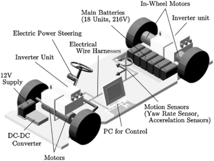
The EV system is shown in Figure 1 [8]. The motor drives the wheel by the transmission to move forward. In this paper, the focus is on wheel and motor. We aim to control the motor to provide the appropriate torque to wheel when the friction between wheel and road is unknown.

Figure 1

The EV system

Figure 2 shows the relation among motor, transmission and wheel. $\omega _m$, $T_m$ and $J_m$ represent the speed, output torque and moment of inertia of the motor, respectively. $\omega _w$, $T_w$ and $J_w$ have the same meanings associated with the wheel. The transmission ratio is i.

Figure 2

The wheel-transmission-motor subsystem

From this figure, we have

$$\omega _m(t)=i\omega _w(t),$$

(44)

$$T_w(t)=iT_m(t).$$

(45)

The model of the motor is given as follows [36]:

$$J_m{\dot{\omega }}_m(t)=\frac{k_t}{R}u(t)-\frac{k_tk_e}{R}\omega _m(t)-B_m\omega _m(t)-T_m(t),$$

(46)

where $k_t$ and $k_e$ are the constants of the motor torque and the electromotive force, respectively, R is the resistance, $B_m$ is the viscous damping coefficients of the motor, u is the control input voltage.

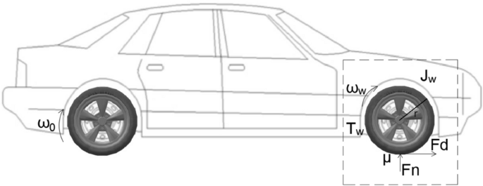
The wheel subsystem is shown in Figure 3. $\omega _w$, $T_w$ and $J_w$ have been shown in Figure 2. $F_n$ is the normal force of wheel, $F_d$ is the driving force, r is the wheel’s radius, $\omega _0$ is the desired speed of the wheel, $\mu$ is the friction coefficient which is regarded as the uncertainty in this paper. The dynamic model of the wheel is given as follows [37, 38]:

$$J_w{\dot{\omega }}_w(t)=T_w(t)-F_d(t)r,$$

(47)

$$F_d(t)=\mu F_n.$$

(48)

Combining Eqs. (44)–(48), the dynamic equation of the whole system can be obtained as follows:

$$J_a{\dot{\omega }}_w(t)=-\left( \frac{k_tk_e}{R}i^2-B_mi^2\right) \omega _w(t)-\mu F_nr+\frac{k_ti}{R}u(t),$$

(49)

where $J_a=J_mi^2+J_w$ is the equivalent moment of the wheel and motor.

Figure 3

The wheel subsystem

Let $x(t)=\omega _w(t)-\omega _0(t)$. Thus, ${\dot{x}}(t)={\dot{\omega }}_w(t)-{\dot{\omega }}_0(t)$. The dynamic equation (49) can be rewritten as

$$\begin{aligned} {\dot{x}}(t)&=-\left( \frac{k_tk_e}{R}+B_m\right) \frac{i^2}{J_a}x(t)\\&\quad +\frac{k_ti}{RJ_a}\left[ u(t)+\frac{R}{k_ti}(-J_a{\dot{\omega }}_0(t)-\left( \frac{k_tk_e}{R}+B_m\right) i^2\omega _0(t)-\mu F_nr)\right] \\&={\widehat{A}}x(t)+{\widehat{B}}(u(t)+{\widehat{v}}(t)). \end{aligned}$$

(50)

Suppose the equivalent moment $J_a$ [39] and the friction coefficient [40] $\mu$ are uncertainties. $J_a={\overline{J}}_a+\Delta J_a(t)$, $\mu ={\overline{\mu }}+\Delta \mu (t)$. Then ${\widehat{A}}=A+\Delta A$, ${\widehat{B}}=B+\Delta B$ and ${\widehat{v}}=v+\Delta v$ with

$$\begin{aligned} A&=-\frac{B_a}{{\overline{J}}_a},\Delta A=\frac{B_a\Delta J_a}{{\overline{J}}_a({\overline{J}}_a+\Delta J_a)},\\ B&=\frac{k_ti}{R{\overline{J}}_a}, \Delta B=-\frac{k_ti\Delta J_a}{R{\overline{J}}_a({\overline{J}}_a+\Delta J_a)},\\ v&=-\frac{R}{k_ti}({\overline{J}}_a{\dot{\omega }}_0+B_a\omega _0+{\overline{\mu }}F_nr),\\ \Delta v&=-\frac{R}{k_ti}(\Delta J_a {\dot{\omega }}_0+\Delta \mu F_nr), \end{aligned}$$

(51)

where $B_a=(k_tk_e/R+B_m)i^2$. By the matching condition, $\Delta A=BD$ and $\Delta B=BE$, we have

$$D=\frac{B_aR}{k_ti}\frac{\Delta J_a}{{\overline{J}}_a+\Delta J_a}, E=-\frac{\Delta J_a}{{\overline{J}}_a+\Delta J_a},$$

(52)

which satisfies the Assumption 3(i).

By Eqs. (51) and (52), the dynamic equation (50) can be rewritten in the form of Eq. (10) with

$$e=Dx+(I+E)\Delta v.$$

(53)

By choosing $Q=I$, $R=I$,

$$\frac{1}{2}\lambda _m(ER^{-1}+R^{-1}E)=E.$$

(54)

Since, $J_a>0$ and ${\overline{J}}_a>0$, as for E,

$$E=-\frac{\Delta J_a}{{\overline{J}}_a+\Delta J_a}=\frac{-\Delta J_a-{\overline{J}}_a+{\overline{J}}_a}{{\overline{J}}_a+\Delta J_a}=-1+\frac{{\overline{J}}_a}{J_a}>-1.$$

(55)

Since $\rho _{E2}\ge 0$, as for ||e||,

$$||e||\leqslant ||D||\,||x||+(I+\rho _{E2})||\Delta v||.$$

(56)

Then, choose $a=||D||$, $b=(1+\rho _{E2})||\Delta v||$. By Eqs. (54)–(56) and choosing $\rho _{E1}=0$, $\rho _{E2}=|\frac{\Delta J_a}{{\overline{J}}_a+\Delta J_a}|$, the Assumption 3(ii) is satisfied.

Remark 8

It is proper that the uncertainties $J_a$ and $\mu$ in the EV model are described by fuzzy set theory. This is because the physical meaning of these two parameters cannot be easily interpreted through the probability theory. Further, the uniform boundedness and uniform ultimate boundedness are ensured for the uncertain EV system based on fuzzy set theory and the Lyapunov approach.

6 Design Procedure

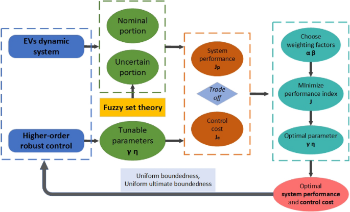
A flowchart is used to summarize the frame this paper as shown in Figure 4.

Figure 4

The frame of EVs system and optimal control design

On the one hand, the dynamical system is established. Furthermore, the uncertain portion of this system is described by fuzzy set theory. On the other hand, a class of novel controls are proposed with two tunable parameters. Then, the cost function which is related to both system performance and control cost is formulated. By minimizing this function, we can obtain the optimal parameters $\gamma$ and $\eta$. Based on that, a better system performance and smaller control cost can be obtained.

7 Simulation Results

The values of the nominal portions in EV system are given as follows: $k_t=2$, $k_e=0.4$, $R=1$, $B_m=0.1$, $i=10$, $F_n=2000$, $r=0.3$, $\omega _0=5$, $\dot{\omega _0}=0$, ${\overline{J}}_a=5$ and ${\overline{\mu }}=0.6$.

For the uncertainties, the amplitude of $\Delta J_a$ is chosen to be “close to 0.5”, the amplitude of $\Delta \mu$ is chosen to be “close to 0.3”. The associated membership functions are given as follows:

$$\phi _{\Delta J_{a}}(\nu )=\left\{ \begin{array}{ll}{2 \nu ,} & \quad{0 \le \nu \le 0.5}, \\ {-2 \nu +2,} & \quad {0.5 \le \nu \le 1},\end{array}\right.$$

(57)

$$\phi _{\Delta \mu }(\nu )=\left\{ \begin{array}{ll}{\frac{10}{3} \nu +1,} & \quad {-0.3 \le \nu \le 0}, \\ {-\frac{10}{3} \nu +1.} & \quad {0 \le \nu \le 0.3}.\end{array}\right.$$

(58)

Then, we choose the crisp initial condition $x(t_s)=x(0)=3$. Thus, $V_s=0.249$. Based on the fuzzy arithmetic, $\kappa _{1\sim 7}$ in Eq. (41) can be obtained.

Table 1 Weighting factors & Optimal parameters & $J_{min}$

By giving different weighting factors $\alpha$ and $\beta$, which means how much we concern about the system performance or control cost, different values of $\gamma$, $\eta$ and $J_{min}$ are obtained by Eqs. (42) and (43). Their values are shown in Table 1. Specifically, the parameters $\alpha$ and $\beta$ are the weighting factors of system performance and control cost, respectively. In the optimization problem, In this optimization problem, a larger $\beta$ value represents that we expect to optimize the control first. At this point, the system will reduce the control cost at the expense of performance. Vice versa. Therefore, in the simulation, by comparing different beta values and control costs, the smaller control at larger beta values is expected to obtain. Finally, the simulations were performed by using $\Delta J_a=0.5|\text {cos}(3t)|$ and $\Delta \mu =0.3\text {sin}(5t)$. LQR is selected for comparison. The reasons for choosing LQR are twofold. First, the LQR is a proven optimal control, which minimizes a performance index including the state and control costs. Second, the LQR is a proven robust control. Many new control methods have been compared with LQR, such as the fuzzy control [41] and the adaptive control [42]. The most common robustness measures attributed to the LQR are a one-half gain reduction in any input channel, an infinite gain amplification in any input channel, or a phase error of plus or minus sixty degrees in any input channel. In addition, there is robustness to uncertainty in the real coefficients of the model and certain nonlinearities, including control switching and saturation [43].

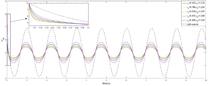
Figure 5 shows the speed of wheel $\omega _w$ histories with different optimal parameters $\gamma$ and $\eta$. LQR control is also plotted as comparison. It shows that the proposed controls are able to render $\omega _w$ in a smaller region than LQR control. From the partial figure, we can find that the proposed controls can stabilize the speed of wheel faster than LQR control as well.

Figure 5

Comparison of control output $\omega _t$ histories

In order to show the system performance more clearly, we define the accumulative error $\Sigma _{\omega }$ as

$$\Sigma _{\omega }=\int ^{t_s}_{0}(\omega _w(t)-\omega _0) \text{d}t.$$

(59)

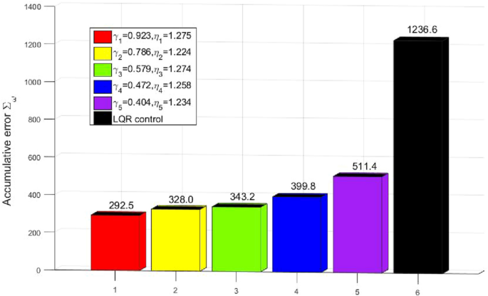
Figure 6 shows the accumulative errors $\Sigma _{\omega }$ under different controls. The accumulative errors of the system under the proposed controls are much more smaller than the accumulative error under LQR control. Furthermore, Figure 5 and Figure 6 show that the performance of the system gets better as the ratio of weighting factors $\alpha /\beta$ becomes larger. Since a larger ratio $\alpha /\beta$ means that we concern more about the system performance than the control cost.

Figure 6

Comparison of accumulative error $\Sigma _{\omega }$

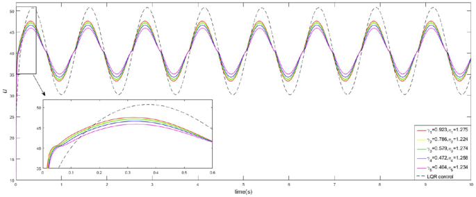
Figure 7 shows the control input u histories with different optimal parameters $\gamma$ and $\eta$. LQR control is also plotted as comparison. It can be seen that the fluctuations of the proposed controls are smaller than the fluctuations of LQR control.

Figure 7

Comparison of control input u histories

Similarly, we define the accumulative control cost $\Sigma _{u}$ as

$$\Sigma _{u}=\int ^{t_s}_{0}u(t) \text{d}t.$$

(60)

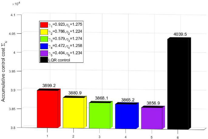
Figure 8 shows the comparison of the control costs with LQR. As shown in this figure, the control efforts with optimal parameters are significantly less than LQR, while demonstrating superior performance. It can be seen that the accumulative control cost decreases as the ratio of weighting factors $\alpha /\beta$ becomes smaller. Since a smaller ratio means that we concern more about the control costs than the system performance.

Figure 8

Comparison of accumulative control cost $\Sigma _{u}$

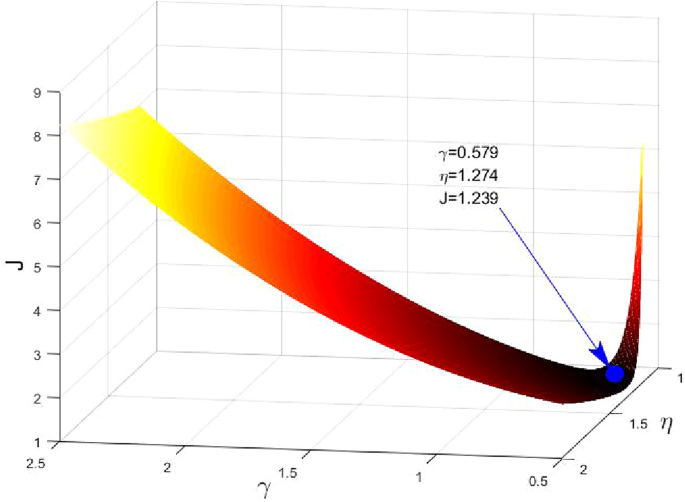
Figure 9 shows the relation between the performance index J, optimal parameters $\gamma$ and $\eta$ when $\alpha =\beta =1$. It verifies the correctness of $J_{min}$ which is obtained by Eqs. (42) and (43).

Figure 9

Relation between J, $\gamma$ and $\eta$ under $\alpha =\beta =1$

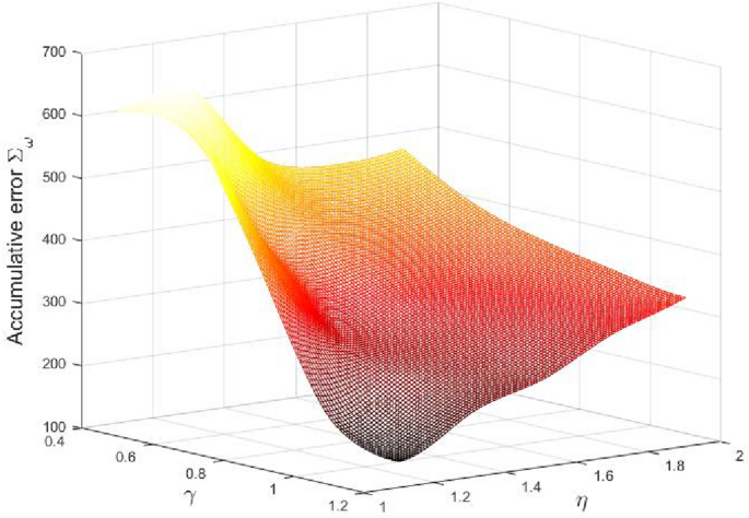
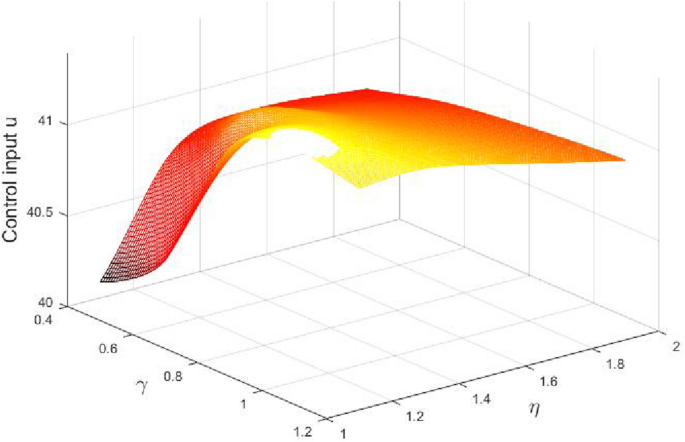
Figure 10 and Figure 11 show the relation between $\Sigma _{\omega }$, u and $\gamma$, $\eta$, respectively. It can be seen the larger $\gamma$ renders better performance and larger control input, and vice verse. However, $\eta$ does not have such monotonicity with $\Sigma _{\omega }$ and u. Thus, $\gamma$ decreases when we concern more about control cost, namely $\alpha /\beta$ decreases while $\eta$ always remains around a certain value as shown in Table 1.

Figure 10

Relation between accumulative error $\Sigma _{\omega }$, $\gamma$ and $\eta$

Figure 11

Relation between control input u, $\gamma$ and $\eta$

8 Conclusions

A class of higher-order robust controls are proposed for EVs. The speed of EVs can be kept stable by these controls when there exists uncertainty. It should be noted that the controls are deterministic based on tunable parameters instead of IF-THEN fuzzy rules. They are able to guarantee uniform boundedness and uniform ultimate boundedness of the system via the Lyapunov minimax approach. Furthermore, the system uncertainty and performance are described by fuzzy set theory. Then, the optimal gain design problem with multi parameters is taken into consideration. A performance index including the tunable parameters $\gamma$ and $\eta$ is presented. By giving different weighting factors of system performance and control cost, the optimal parameters $\gamma$ and $\eta$ can be solved by minimizing the performance index J. The results of this paper demonstrate that the newly proposed high-order robust controller can be applied to the anti-skid control of electric vehicles. In addition, the optimization method proposed in this paper can find the optimal parameters of the controller to achieve better system performance.

References

C Chan. The past, present and future of electric vehicle development. Proceedings of the IEEE 1999 International Conference on Power Electronics and Drive Systems, 1999, 1: 11–13.
S-I Sakai, Y Hori. Advantage of electric motor for anti skid control of electric vehicle. EPE Journal, 2001, 11(4): 26–32.
L Li, S Kodama, Y Hori. Anti-skid control for EV using dynamic model error based on back-emf observer. The 30th Annual Conference of IEEE Industrial Electronics Society, 2004, 2: 1700–1704.
B Subudhi, S S Ge. Sliding-mode-observer-based adaptive slip ratio control for electric and hybrid vehicles. IEEE Transactions on Intelligent Transportation Systems, 2012, 13(4): 1617–1626.
T Kanou, H Fujimoto. Slip-ratio based yaw-rate control with driving stiffness identification for electric vehicle. Proceedings of 9th International Symposium on Advanced Vehicle Control, 2008: 786–791.
S Li, K Nakamura, T Kawabe, et al. A sliding mode control for slip ratio of electric vehicle. 2012 Proceedings of SICE Annual Conference (SICE), 2012: 1974–1979.
H Fujimoto, T Saito, T Noguchi. Motion stabilization control of electric vehicle under snowy conditions based on yaw-moment observer. The 8th IEEE International Workshop on Advanced Motion Control, 2004: 35–40.
Y Hori. Future vehicle driven by electricity and control-research on four wheel motored. The 7th International Workshop on Advanced Motion Control Proceedings, 2002: 1–14.
D Yin, S Oh, Y Hori. A novel traction control for EV based on maximum transmissible torque estimation. IEEE Transactions on Industrial Electronics, 2009, 56(6): 2086–2094.
X Peng, H Zhe, G Guifang, et al. Anti-slip regulation of electric vehicle without speed sensor. 2009 IEEE International Symposium on Industrial Electronics, 2009: 222–227.
K Xu, G Xu, W Li, et al. Anti-skid for electric vehicles based on sliding mode control with novel structure. 2011 IEEE International Conference on Information and Automation, 2011: 650–655.
T Augustin, F P Coolen, G De Cooman, et al. Introduction to imprecise probabilities. John Wiley & Sons, New Jersey, 2014.
D Dubois, H Prade. Possibility theory and its applications: Where do we stand? In: Springer handbook of computational intelligence, Springer, New York, 2015: 31–60.
R Kalman. Randomness reexamined. Modeling, Identification and Control, 1994, 15(3): 141–151.
L A Zadeh. Fuzzy sets. Information and Control, 1965, 8(3): 338–353.
J C R Alcantud, S Díaz. Rational fuzzy and sequential fuzzy choice. Fuzzy Sets and Systems, 2017, 315: 76–98.
A Khastan, Z Alijani. On the new solutions to the fuzzy difference equation xn+ 1= a+ bxn. Fuzzy Sets and Systems, 2019, 358: 64–83.
M Sugeno, G Kang. Structure identification of fuzzy model. Fuzzy Sets & Systems, 1988, 28(1): 15–33.
T Takagi, M Sugeno. Fuzzy identification of systems and its applications to modeling and control. IEEE Transactions on Systems, Man, and Cybernetics, 1985, (1): 116–132.
C S Tseng, B S Chen, H J Uang. Fuzzy tracking control design for nonlinear dynamic systems via TS fuzzy model. IEEE Transactions on Fuzzy Systems, 2001, 9(3): 381–392.
Z Zhang, L Chong, C Bing. New stability and stabilization conditions for T-S fuzzy systems with time delay. Fuzzy Sets & Systems, 2015, 263(C): 82–91.
X P Guan, C L Chen. Delay-dependent guaranteed cost control for TS fuzzy systems with time delays. IEEE Transactions on Fuzzy Systems, 2004, 12(2): 236–249.
Y-H Chen. A new approach to the control design of fuzzy dynamical systems. Journal of Dynamic Systems, Measurement, and Control, 2011, 133(6): 1–9.
J Han, Y-H Chen, X Zhao, et al. Optimal design for robust control of uncertain flexible joint manipulators: A fuzzy dynamical system approach. International Journal of Control, 2018, 91(4): 937–951.
H Sun, H Zhao, K Huang, et al. A fuzzy approach for optimal robust control design of an automotive electronic throttle system. IEEE Transactions on Fuzzy Systems, 2017, 26(2): 694–704.
S Gutman. Uncertain dynamical systems–A Lyapunov min-max approach. IEEE Transactions on Automatic Control, 1979, 24(3): 437–443.
G J Klir, B Yuan. Fuzzy sets and fuzzy logic: Theory and applications. Prentice Hall PTR, New Jersey, 1995.
Y H Chen. Performance analysis of controlled uncertain systems. Dynamics and Control, 1996, 6(2): 131–142.
J Bezdek. Special issue on fuzziness vs. probability—the n-th round. IEEE Transactions on Fuzzy Systems, 1994, 2(1): 1–42.
J Huang, Y H Chen, A Cheng. Robust control for fuzzy dynamical systems: Uniform ultimate boundedness and optimality. IEEE Transactions on Fuzzy Systems, 2012, 20(6): 1022–1031.
H Sun, R Yu, Y H Chen, et al. Optimal design of robust control for fuzzy mechanical systems: performance-based leakage and confidence-index measure. IEEE Transactions on Fuzzy Systems, 2019, 27(7): 1441–1455.
J Xu, Y H Chen, H Guo. Fractional robust control design for fuzzy dynamical systems: An optimal approach. Journal of Intelligent and Fuzzy Systems, 2015, 29(2): 553–569.
M J Corless. Control of uncertain nonlinear systems. Journal of Dynamic Systems, Measurement, and Control, 1993, 115(2B): 362–372.
G Leitmann. On one approach to the control of uncertain systems. Proceedings of 1994 33rd IEEE Conference on Decision and Control, 1994, 3: 2112–2116.
J K Hale. Functional differential equations. In: Analytic theory of differential equations, Springer, New York, 1971: 9–22.
X Jiao, J Zhang, T Shen. An adaptive servo control strategy for automotive electronic throttle and experimental validation. IEEE Transactions on Industrial Electronics, 2014, 61(11): 6275–6284.
T D Gillespie. Fundamentals of vehicle dynamics. Technical report, SAE Technical Paper, 1992.
Z Cai, C Ma, Q Zhao. Acceleration-to-torque ratio based anti-skid control for electric vehicles. Proceedings of 2010 IEEE/ASME International Conference on Mechatronic and Embedded Systems and Applications, 2010: 577–581.
W Xie, D Cabecinhas, R Cunha, et al. Adaptive backstepping control of a quadcopter with uncertain vehicle mass, moment of inertia, and disturbances. IEEE Transactions on Industrial Electronics, 2021, 1–1, https://doi.org/10.1109/TIE.2021.3055181.
A Guerine, A El Hami, L Walha, et al. Dynamic response of a spur gear system with uncertain friction coefficient. Advances in Engineering Software, 2018, 120: 45–54.
N S Bhangal. Design and performance of lqr and lqr based fuzzy controller for double inverted pendulum system. Journal of Image and Graphics, 2013, 1(3): 143–146 (2013)
A A Ghaffar, T Richardson. Model reference adaptive control and lqr control for quadrotor with parametric uncertainties. International Journal of Mechanical and Mechatronics Engineering, 2015, 9(2): 244–250.
J C Doyle, B A Francis, A R Tannenbaum. Feedback control theory. Courier Corporation, North Chelmsford, 2013.
Acknowledgements
Not applicable.
Funding
Supported by China Scholarship Council (Grant No. 201806690019), Fundamental Research Funds for Chinese Central Universities (Grant No. 300102258306), and Anhui Provincial Natural Science Foundation of China (Grant No. 1908085QE194).
Author information
Authors and Affiliations
Contributions
CL: Software, writing the original draft, formal analysis and simulations. YC: Conceptualization, methodology, writing and review. KH: Data curation and supervision. HZ: Resources, project administration. All authors read and approved the final manuscript.
Authors’ Information
Chenming Li (1993) is currently pursuing the Ph.D. degree with the School of Mechanical Engineering, Hefei University of Technology, China. He is also a Visiting Scholar with the George W. Woodruff School of Mechanical Engineering, Georgia Institute of Technology, USA. His research interests include mechanical system dynamics, optimal design of robust control, adaptive robust control, and fuzzy engineering.
Ye-Hwa Chen (1956) received the Ph.D. degree in mechanical engineering from the University of California at Berkeley, USA, in 1985. He is currently a Professor with the National Engineering Laboratory for Highway Maintenance Equipment, Chang’an University, China, and also with the George W. Woodruff School of Mechanical Engineering, Georgia Institute of Technology, USA. His research interests include advanced control methods for mechanical systems, fuzzy engineering, adaptive robust control, and uncertainty management.
Kang Huang (1968) received the Ph.D. degree in mechanical engineering from Hefei University of Technology, China, in 2002. He is currently a Professor with the School of Mechanical Engineering, Hefei University of Technology, China. His research interests include vehicle system dynamics, robotics and vehicle active safety technology.
Han Zhao (1957) received the Ph.D. degree in mechanical engineering from Aalborg University, Denmark, in 1990. He is currently a Professor with the School of Mechanical Engineering, Hefei University of Technology, China. His research interests include mechanical system dynamics, vehicle system dynamics, optimal control, adaptive robust control, and fuzzy engineering.
Corresponding author
Ethics declarations
Competing Interests
The authors declare that they have no competing interests.
Rights and permissions
Open Access This article is licensed under a Creative Commons Attribution 4.0 International License, which permits use, sharing, adaptation, distribution and reproduction in any medium or format, as long as you give appropriate credit to the original author(s) and the source, provide a link to the Creative Commons licence, and indicate if changes were made. The images or other third party material in this article are included in the article's Creative Commons licence, unless indicated otherwise in a credit line to the material. If material is not included in the article's Creative Commons licence and your intended use is not permitted by statutory regulation or exceeds the permitted use, you will need to obtain permission directly from the copyright holder. To view a copy of this licence, visit http://creativecommons.org/licenses/by/4.0/.
About this article
Cite this article
Li, C., Zhao, H., Huang, K. et al. Optimal Design for Anti-Skid Control of Electric Vehicles by Fuzzy Approach. Chin. J. Mech. Eng. 34, 125 (2021). https://doi.org/10.1186/s10033-021-00642-8
Received:
Revised:
Accepted:
Published:
DOI: https://doi.org/10.1186/s10033-021-00642-8