- Original Article
- Open access
- Published:
Optimum Seeking of Redundant Actuators for M-RCM 3-UPU Parallel Mechanism
Chinese Journal of Mechanical Engineering volume 34, Article number: 121 (2021)
Abstract
The singularity problem brings troubles to the design and application for the parallel mechanism. Currently, redundant actuation is one of the useful methods to solve this singularity problem. However, faced to the numerous joints in a parallel mechanism, how to make a quantitative criterion of seeking the most efficient joints added actuators for letting the mechanism passes through singularity is a necessarily open issue. This paper focuses on a 2R1T 3-UPU (U for universal joint and P for prismatic joint) parallel mechanism (PM) with two rotational and one translational (2R1T) degrees of freedom (DOFs) and the ability of multiple remote centers of motion (M-RCM). The singularity analysis based on the indexes of motion/force transmissibility and constraint shows that this PM has transmission singularity, constraint singularity, mixed singularity and limb singularity. To solve these singular problems, the quantifiable redundancy transmission index (RTI) and the redundancy constraint index (RCI) are proposed for optimum seeking of redundant actuators for this PM. Then the appropriate redundant actuators are selected and the working scheme for redundant actuators near the corresponding singular configuration are given to help the PM passes through the singularity. This research proposes a quantitative criterion to optimum seeking of redundant actuators for the parallel mechanism to solve its singularity.
1 Introduction
The RCM (remote center of motion) mechanism, which can rotate around a fixed point far away from the mechanism itself [1], is mostly used in minimally invasive surgery robots at the beginning [2,3,4,5]. There are two main approaches to achieve this [6]: the first is the redundant degrees of freedom (DOF), which requires additional control means, the second is by the constraints of the mechanism itself. The latter can be divided into the following types [7, 8]: ring guide, parallelogram link, spherical link, planar linkage, belt drive, multi-stage gear and parallel mechanism [9], etc.
This kind of rotation around the remote center is not only required in minimally invasive surgery, but also of great significance in metal cutting. It can be linked to an important function of five axis machine tool: tool tip follow, also known as Rotated Tool Center Point (RTCP) or tool center point management (TCPM) [10, 11]. In the five-axis machining, because the rotational center of the tool is not at the tool nose, additional translation of tool nose is generated, which makes the control point of the CNC system often not coincide with the tool nose. Therefore, the CNC system should control the translational axis automatically to ensure that the tool center point and the actual contact point between the tool and the workpiece surface remain unchanged. In essence, it is also the demand of the mechanism for RCM function (rotation around the tool tip). However, for the current series machine tool and hybrid machine tool, the approach to realize this motion belongs to the first one mentioned above.
In the previous work [12, 13], a 2R1T 3-UPU PM is studied, which can make a two-dimensional fixed-point rotation around any point in its “constraint plane”. By adjusting the geometric parameters of the PM, the “constraint plane” can be placed outside the mechanism to realize multiple remote motion centers, which can be called the M-RCM mechanism.
Based on the 2R1T M-RCM 3-UPU PM in series with a 2-DOF mobile platform, a hybrid machine tool can be designed to realize the RTCP function without additional translation for real-time compensation. This undoubtedly shortens the length of the kinematic chain during the RTCP, improves the accuracy of the machine tool, and reduces the difficulty of calibration. However, the singularity problem limits its workspace and performance, so the solution for the singularity of this PM needs to be explored.
For the PMs, the main solution for singularity is redundant actuation [14]. Besides, the application of redundant actuators can also optimize the driving force and load distribution of each joint [15, 16], increase the stiffness [17], improve the bearing capacity [14], and reduce the motion error caused by the clearance of the joint [18, 19]. The PMs with redundant actuation can be divided into two types [16]: (1) The limb redundancy which is to add one or more driven limbs with the original DOF characteristic of the mechanism unchanged. (2) The joint redundancy in the limb which is to convert one or more passive joints in one or more limbs into actuator with the original DOF characteristic of the mechanism unchanged. To avoid the impact of extra limbs on the workspace and reduce the cost, this paper will focus on the latter type. However, there are usually many joints in the limbs of PMs. How to select the optimal redundant driving joints to make the mechanism pass through the singular configuration better is a key to the design and application of this M-RCM 3-UPU PM.
Ball [20] according to the wrench and twist, firstly propose the virtual coefficient which can describe the power between the instantaneous motion of the rigid body and the force on it. Then, this theory has been constantly improved in the process of development [21, 22]. Liu et al. [23,24,25] defined the motion/force transfer index and the motion/force constraint index in DOF space and constraint space respectively to evaluate motion/force transmission and constraint performance qualitatively and quantitatively for the non-redundantly actuated PMs. And these indexes can also be used for singularity analysis [26,27,28]. For the performance analysis of redundantly actuated PMs, the solution is to simplify the mechanism to multiple non-redundantly actuated one by the permutation and combination of each actuator and to formulate corresponding indexes [29,30,31]. However, when the PM with joint redundancy in the limb has multiple redundant actuator combinations, how to select the most suitable combination of actuator joints to make the mechanism pass the singular configuration best is an open issue.
This paper focuses on this issue and is organized as follows: Section 2 gives the description of an M-RCM 3-UPU PM and its model of inverse kinematics. Section 3 analyzes the singularity problem of this 3-UPU PM based on the indexes of motion/force transmissibility and constraint, and the types of singularity are classified. In Section 4, the corresponding performance index of the redundant actuator is proposed for different types of singularity, and the two combinations of the redundant actuator are analyzed and compared. Then the optimum seeking of redundant actuation for this PM is given. Conclusions are presented in Section 5.
2 Description of the Mechanism
2.1 M-RCM 3-UPU Parallel Mechanism
The structure diagram of M-RCM 3-UPU parallel mechanism is shown in Figure 1. It is composed of the base platform (equilateral triangle ∆A1A2A3), mobile platform (equilateral triangle ∆B1B2B3) and three limbs of UPU distributed symmetrically at 120°. Each limb contains two universal joints and one prismatic joint. For the convenience of description, the upper and lower universal joints in each limb are divided into two orthogonal revolute joints of Single-DOF and are named respectively. In the lower U joint of the ith (i = 1, 2, 3) limb, the R joint directly connected to the base platform is named Ri1, and another R joint that is perpendicular to Ri1 is named Ri2. The P joint is named Pi3. In the upper U joint, the R joint directly connected to the mobile platform is named Ri5, and another R joint that is perpendicular to Ri5 is named Ri4. The axes of Ri2 and Ri4 are parallel. The angle between the axis of Ri1 and the base platform is denoted by θ, which is the same as that between the axis of Ri5 and the mobile platform. Meanwhile, the axes of Ri1 and Ri5 in each limb intersect at point Mi, and a plane m is determined by M1, M2, and M3. A1, A2, A3 are the center points of the lower U joint, and B1, B2, B3 are the center points of the upper U joint.

Structure diagram of M-RCM 3-UPU PM
When the joints in the UPU limb satisfy the above geometric conditions, each UPU limb provides a constraint force to the mobile platform. The constraint force of the ith limb is denoted by $ci, passing through point Mi and being parallel with the axis of Ri2. In the non-singular configuration, the three constraints provided by the three UPU limbs are always located in plane m (the plane m can also be called constraint plane), which limits one rotational DOF and two translational DOF for the mechanism. Therefore, the DOF of the mechanism is 2R1T. The mobile platform can rotate continuously around any axis in the constraint plane m, and can also translate along the normal direction of the constraint plane m. Because the output motion of the mechanism is only pure rotation and pure translation, there is no parasitic motion [12]. By adjusting the geometric parameters of the mechanism, the constraint plane can be placed up away from the mobile platform as shown in Figure 1. At this time, the mechanism has multiple remote motion centers on plane m, which can be called M-RCM 3-UPU PM.
The global coordinate system {Ro} is attached on the base at point O which is the center of the base platform A1A2A3. The X-axis is parallel with the base side A1A3 and the Z-axis is vertical to the base. The Y-axis is defined by the right-hand rule. The mobile coordinate system {Rp} is attached on the mobile platform at point P, which is the center of the mobile platform B1B2B3. The x-axis is parallel with the side B1B3 and the z-axis is vertical to the mobile platform. The y-axis is defined by the right-hand rule. There are three key structural parameters of the mechanism, which are the circumscribed radius of the base platform \(R = \left| {{\varvec{OA}}_{i} } \right|\), the circumscribed radius of the mobile platform \(r = \left| {{\varvec{PB}}_{i} } \right|\), and the angle θ.
2.2 Inverse Kinematics
The mobility of this PM is 2R1T, as shown in Figure 2. Its configuration can be described by two angles α, β, and the distance s. The definitions of these parameters are as follows: The projection of the positive direction of z-axis on the XOY plane of {Ro} is a vector denoted by n. The angle between n and the positive direction of X-axis is α. The angle between the positive direction of z-axis and Z-axis is β. Meanwhile, s represents the distance between P and O. The change between different configurations of this mechanism can be considered that the mobile platform rotates β about k and translates from O to P.

Inverse kinematics of M-RCM 3-UPU
Given α, β and s, the inverse kinematics of this mechanism is to solve the length of three prismatic joints. According to the previous work [12], when the mobile platform is enlarged to the same size as the fixed platform triangle along the axes of R15, R25 and R35, a virtual mobile platform named C1C2C3 can be obtained. At this time, the virtual mobile platform C1C2C3 is always symmetrical to the base platform A1A2A3 concerning the constraint plane m regardless of the configuration of the mechanism. Since the magnification from the mobile platform to the virtual mobile platform is fixed and known, these two platforms can be regarded as fixed connection, that is to say, the rotation parameters α and β of the virtual mobile platform are consistent with those of the mobile platform, and only the distances d and s from the respective center points to the base platform are different.
Based on the aforesaid relation, set \(h = \left| {{\varvec{PP^{\prime}}}} \right|\), and in the trapezoid \(PB_{2} C_{2} P^{\prime}\), there is
The intersection point of Z-axis and the constraint plane m is marked as T. According to the symmetry relationship between A1A2A3 and C1C2C3, we can know that \(\left| {{\varvec{TO}}} \right| = \left| {{\varvec{TP^{\prime}}}} \right|\), then
As shown in Figure 2, the relationship between s and d can be obtained by cosine law in \(\triangle OPP^{\prime}\)
When s is known and d can be obtained by Eq. (3), the coordinates of \(P^{\prime}\) in {Ro} can be expressed by
Here, a vector k can be defined by \({\varvec{k}} = {\varvec{Z}} \times {\varvec{n}}\). Since, the axes of {Rp} and coordinate system of virtual moving platform {Rp’} are parallel, their rotation matrices relative to {RO} are both equivalents to rotating β around the vector k.
The coordinates of \(P^{\prime}\) in {Rp} is \(\left[ {\begin{array}{*{20}c} 0 & 0 & h \\ \end{array} } \right]^{{\text{T}}}\), then the coordinates of \(P^{\prime}\) in {RO} can be expressed by
The coordinates of Bi in {Rp} are easy to be obtained, and its coordinates can be calculated in {RO} by
Finally, the length of three prismatic joints can be obtained by the following equation
3 Singularity Analysis
This kind of 3-UPU PM needs a larger angle θ in M-RCM working configuration, which means that the workspace is easily limited by singularity [12]. The traditional method of singularity analysis is mainly focused on whether the Jacobian matrix of the mechanism is reduced in rank or whether the constraint/actuation screw system of the mechanism is linearly correlated, which is difficult to quantitatively evaluate the performance of the mechanism at the singularity configuration or nearby. The motion/force transmissibility and motion/constraint transmissibility can also be used to analyze the singularity of mechanism and have advantages in the quantitative evaluation of the kinematic performance of the mechanism. To compare the influence of various redundant actuation modes on the ability of the mechanism passing through the singular configuration, the motion/force transmissibility and constraint are used here as the index to analyze the singularity of the mechanism.
3.1 Indexes of Motion/Force Transmissibility and Constraint
Firstly, the non-redundant mechanism is considered, and only the prismatic joint of each limb is taken as the actuator. The UPU limb is shown in Figure 3. The unit twist describing the jth 1-DoF joint in the ith limb is denoted by $ij (0 < i ≤ 3, 0 < j ≤ 5). All the unit twists of joint in the ith UPU limb constitute its limb twist system that is denoted by {TLi}, then

UPU limb
Based on the screw theory, when the twists in {TLi} are linearly independent with each other, a screw $ci which is reciprocal to all the unit twists in {TLi}, can be obtained by
The constraint wrench screw (CWS) $ci is a line vector provide by the ith UPU limb to the mobile platform and acts on Mi point with the direction parallel to the axis of $i2.
When the driving joint P is locked, the rank of {TLi} decreases due to the lack of the corresponding motion screw of the joint P. In addition to the CWS, there will be a new wrench which is reciprocal to all the twist in the rank reduced limb twist system and is linearly independent with CWS $ci, being denoted by $Ti:
As the UPU limb shown in Figure 3, according to Eq. (11), $Ti can be obtained to be a line vector passing through point Ai and be collinear with the axis of the prismatic joint. $Ti is the transmission wrench screw (TWS) and can also be called the actuation force screw.
Similarly, if the kth (k = 1, 2, 4, 5) joints other than the driving joint P in the ith limb are locked (the rest joints including the P joint remain unchanged), there will be another wrench which is reciprocal to all the twist in the rank reduced limb twist system, and it is linearly independent with the CWS $ci, which is denoted by $aik. $aik satisfy the following formula:
When the revolute joint Ri1 is locked, the corresponding $a11 obtained by Eq. (12) is a couple passing through point Bi. The real unit and dual unit of $a11 are represented by \({\varvec{S}}_{a11}\) and \({\varvec{S}}_{a11}^{0}\) respectively, and \({\varvec{S}}_{a11}^{0}\) satisfies the following relationship
When the revolute joint Ri2 is locked, the corresponding $ai2 obtained by Eq. (12) is a line vector passing through point Bi and satisfies the following relationship
Meanwhile, \({\varvec{S}}_{ai2}\) intersects with \({\varvec{S}}_{i1}\).
When the revolute joint Ri4 is locked, the corresponding $ai4 obtained by Eq. (12) is a line vector passing through point Ai and satisfies the following relationship
Meanwhile, \({\varvec{S}}_{ai4}\) intersects with \({\varvec{S}}_{i5}\).
When the revolute joint Ri5 is locked, the corresponding $ai5 obtained by Eq. (12) is a couple passing through point Ai and satisfy the following relationship
If the driving joint is determined, the input twist screw (ITS) of the limb is consistent with the kinematic twist of the corresponding joint, which is easy to obtain:
The output twist screw (OTS) is the unit instantaneous motion generated by the mobile platform only through the driving of the ith limb with the driving joint outside the ith limb locked, which is recorded as $oi. In other words, only the TWS of the ith limb can work on the mobile platform of the mechanism in this situation, and the TWS of the rest limbs is also regarded as the constraint to the mechanism. $oi can be obtained according to the following formula:
The restricted twist screw (RTS) of the ith limb, denoted by $rti, refers to the motion that cannot be caused by this ith limb no matter the actuator added to any joint in the limb. According to the Eqs. (11)‒(16), the driving force subspace of the ith limb that denoted by {WAi} can be determined as
$rti is reciprocal to all the unit twists in {WAi} and based on the screw theory, $rti is a couple in the same directions of $ai2 and $ci.
The output restricted twist screw (ORTS) that denoted by \(\Delta /\!\!\!{{\varvec{S}}}_{Oi}\) is the unit motion screw of the mechanism that is allowed to occur when the CWS provided by ith limb is set free, with the CWS of the rest limbs and the TWS of all limbs unchanged. \(\Delta /\!\!\!{{\varvec{S}}}_{Oi}\) can be obtained by the following equation
If the motion of a rigid body is a unit twist $1, the power of a unit wrench $2 to this body can be expressed by the reciprocal product between $1 and $2. Then the following indexes of performance will be easier to understand.
-
(1)
Input transmission index (ITI)
When the PM is non-redundant actuated, only the P joints in the three limbs are selected as the actuators. ITI represents the ratio of instantaneous power between TWS $Ti (a line vector for this UPU limb) and ITS $Ii (a couple for this UPU limb) to its corresponding potential maximum power which can be obtained from the following formula:
$$\mu_{i} = \frac{{\left| {/\!\!\!{{\varvec{S}}}_{Ti} \circ /\!\!\!{{\varvec{S}}}_{Ii} } \right|}}{{\left| {/\!\!\!{{\varvec{S}}}_{Ti} \circ /\!\!\!{{\varvec{S}}}_{Ii} } \right|_{\max } }} = \left| {{\text{cos}}\varphi_{i} } \right|.$$(21)Since the axis of $Ti is always in the same direction as that of $Ii, and the angle φi between the two axes is 0, ITI for this PM is always 1.
-
(2)
Output transmission index (OTI)
OTI represents the ratio of instantaneous power between TWS $Ti (a line vector for this UPU limb) and OTS $oi to its corresponding potential maximum power. Take the first limb for example. As shown in Figure 4, point E1 and point F1 are the intersections of $T2 and $T3 with the constraint plane m, respectively. According to Eq. (18), it can be obtained that $O1 is a line vector with E1F1 as the axis and a zero pitch. Then OTI can be obtained from the following formula:
$$\eta_{i} = \frac{{\left| {/\!\!\!{{\varvec{S}}}_{Ti} \circ /\!\!\!{{\varvec{S}}}_{Oi} } \right|}}{{\left| {/\!\!\!{{\varvec{S}}}_{Ti} \circ /\!\!\!{{\varvec{S}}}_{Oi} } \right|_{\max } }}{ = }\frac{{\left| {d_{1i} \sin \sigma } \right|}}{{\left| {d_{1i\max } } \right|}},$$(22)where the definition of d1i and d1imax is taken the first limb for example.
Figure 4 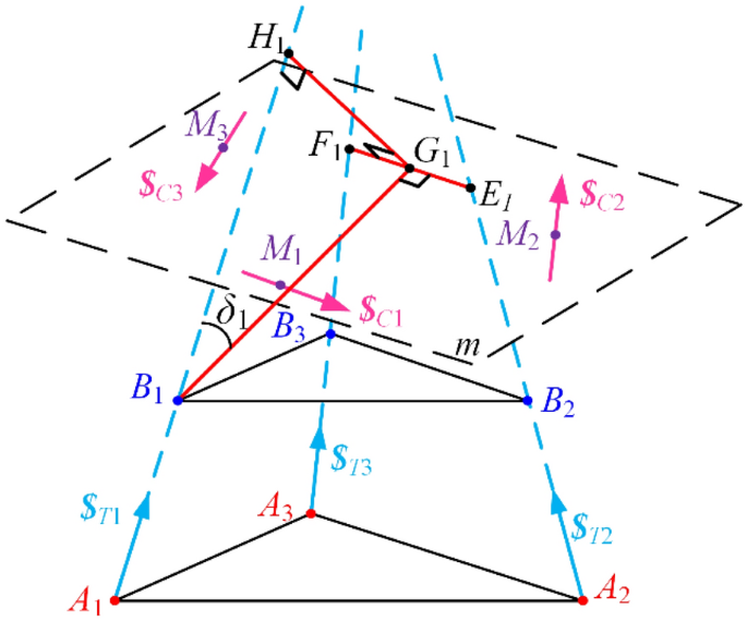
Calculation for OTI
As shown in Figure 4, d11 is the distance of the common perpendicular (G1H1) between $T1 and $O1. So, \(d_{11} = \left| {G_{1} H_{1} } \right|\). Since the point of action for $T1 to the mobile platform is always B1, the corresponding potential maximum power is equal to the distance from B1 to the axis of $O1. So \(d_{11\max } = \left| {B_{1} G_{1} } \right|\). For the first limb, Eq. (22) can be simplified by
$$\eta_{{1}} { = }\frac{{\left| {d_{{1{1}}} \sin \sigma } \right|}}{{\left| {d_{11\max } } \right|}}{ = }\frac{{\left| {{\varvec{G}}_{1} {\varvec{H}}_{1} } \right|}}{{\left| {{\varvec{B}}_{1} {\varvec{G}}_{1} } \right|}} = \sin \delta_{1} ,$$(23)where δ1 is the angle between the axis of $T1 and B1G1.
-
(3)
Input constraint index (ICI)
ICI represents the ratio of instantaneous power between CWS $Ci (a line vector for this UPU limb) and RTS $rti (a couple for this UPU limb) to its corresponding potential maximum power which can be obtained from the following formula:
$$\varepsilon_{i} = \frac{{\left| {/\!\!\!{{\varvec{S}}}_{Ci} \circ /\!\!\!{{\varvec{S}}}_{rti} } \right|}}{{\left| {/\!\!\!{{\varvec{S}}}_{Ci} \circ /\!\!\!{{\varvec{S}}}_{rti} } \right|_{\max } }}{ = }\left| {\cos \psi } \right|.$$(24)Since the axis of $Ci is always in the same direction as that of $rti, and the angle ψi between the two axes is zero, ICI for this PM is always 1.
-
(4)
Output constraint index (OCI)
OCI represents the ratio of instantaneous power between CWS $Ci (a line vector for this UPU limb) and ORTS \(\Delta /\!\!\!{{\varvec{S}}}_{Oi}\) to its corresponding potential maximum power which can be obtained from the following formula:
$$\tau_{i} = \frac{{\left| {/\!\!\!{{\varvec{S}}}_{Ci} \circ \Delta /\!\!\!{{\varvec{S}}}_{Oi} } \right|}}{{\left| {/\!\!\!{{\varvec{S}}}_{Ci} \circ \Delta /\!\!\!{{\varvec{S}}}_{Oi} } \right|_{\max } }}{ = }\frac{{\left| {h_{Oi} \cos \gamma_{i} - d_{2i} \sin \gamma_{i} } \right|}}{{\sqrt {h_{Oi}^{2} + d_{2i\max }^{2} } }},$$(25)where hoi is the pitch of \(\Delta /\!\!\!{{\varvec{S}}}_{Oi}\), γi is the angle between $Ci and \(\Delta /\!\!\!{{\varvec{S}}}_{Oi}\), d2i is the distance of common perpendicular between $Ci and \(\Delta /\!\!\!{{\varvec{S}}}_{Oi}\), and d2imax is the distance of perpendicular between Mi (which is the point of act for $Ci) and \(\Delta /\!\!\!{{\varvec{S}}}_{Oi}\).
According to the above indexes, local transmission index (LTI) κ and total constraint index (TCI) λ can be established to evaluate the performance of the whole mechanism
$$\begin{gathered} \kappa = \min \left\{ {\mu_{i} ,\eta_{i} } \right\}, \, i = 1,2,3, \hfill \\ \lambda = \min \left\{ {\varepsilon_{i} ,\tau_{i} } \right\}, \, i = 1,2,3. \hfill \\ \end{gathered}$$(26)

3.2 Singularity Analysis Based on the Indexes of Performance and Screw Theory
According to the LTI and TCI obtained in Section 3.1, the values of κ and λ are related to the configuration of the mechanism, and all in the range of [0, 1]. The larger the value of κ and λ, the better the performance of force/motion transmission and constraint respectively. When κ or λ becomes zero, the mechanism comes to the singular configuration. As shown in Figure 1, the structure parameters are R = 100 mm, r = 50 mm, θ=80°. Set s = 170 mm, and the LTI contour map of the mechanism is drawn with α and β as the axes of polar coordinates, as shown in Figure 5. According to the color bar of the legend, the closer the contour color is to blue, the smaller the κ of the mechanism is. The closer the contour color is to yellow, the greater the κ of the mechanism is.

Calculation for OTI
As shown in Figure 5, according to the trend of color change, κ of the mechanism may become zero between two adjacent contour lines that κ = 0.05, that is to say, there is a singular configuration near β = 35°. By further reducing the search step, we can get a singular configuration of the mechanism with α = 90°, β = 34.83° and s = 170 mm, as shown in Figure 6. At this time, the OTI index of limb 2 is \(\eta_{2} = 0\) (less than 10−5 is regarded as zero), and the axis of TWS $T2 intersects the axis of OTS $O2 of mobile platform, so $T2 is unable to work on $O2. Judging from the correlation of the screw system analysis, according to Eq. (18), $O2 is the line vector with E2F2 as the axis, and intersects with the CWS $C1, $C3 and the TWS $T1, $T2, $T3, and it is parallel to the CWS $C2. In other words, under this singular configuration, when the three driving joints P are locked, the instantaneous rotational DOF with E2F2 as the axis is still free.

Transmission singularity
Set s = 85 mm, and the TCI contour performance map of the mechanism is drawn, as shown in Figure 7. According to the color bar of the legend, the closer the contour color is to black, the smaller the λ of the mechanism is, and the closer the color is to white, the greater the λ of the mechanism. According to the trend of color change, λ of the mechanism may become zero between two adjacent contour lines that λ = 0.09, that is to say, there is a singular configuration near β = 20°.

Contour map of TCI
By further reducing the search step, we can get a singular configuration of the mechanism with α = 90°, β = 19.70°, s = 170 mm, as shown in Figure 8. The OCI index of limb 2 is τ2 = 0, and the CWS $C2 cannot work on the ORTS \(\Delta /\!\!\!{{\varvec{S}}}_{Oi}\). This is consistent with the analysis results in Ref. [12]. Since the three constraint forces meet at one point in the plane m, and the constrained screw system is reduced in rank, the rotational DOF of the mechanism with axis passing through M2 and perpendicular to plane m is added.

Constraint singularity
It can also be seen from Figure 7 that the λ of the mechanism is extremely unstable when β = 20°, α = 30°, 150° and 270°. Compared with the analysis results in Ref. [12], this goes against a prerequisite for the performance analysis of motion/force constraint, which is the motion screws of the joints in the limb are independent of each other.
This kind of singular configuration is due to the coincidence of the axes of the two revolute joints in the upper and lower U joints of the same limb, resulting in the local DOF for the limb rotating around the axis of the prismatic joint, as shown in Figure 9.

Limb singularity
To analyze the relationship between the singular configuration and s (the center distance of the mobile platform and the base), and keep the moving platform and the fixed platform parallel, the relationship between LTI, TCI and s is drawn, as shown in Figure 10. It can be found that when s is at 94 mm, LTI and TCI become zero at the same time, which means that the transmission singularity and the constraint singularity occur at the same time, which can also be called mixed singularity. When the mixed singularity occurs, the intersection point Q of the three TWSs just falls on the constraint plane m, as shown in Figure 11. According to the screw theory, any rotation whose axis at plane m passes through Q cannot be limited, and the mechanism is out of control.

Relationship between TCI/LTI and s

Mixed singularity
Because the geometric relationship of the mechanism is very clear in the case of mixed singularity, the configuration of mixed singularity can be deduced as follows:
4 Redundant Actuation and Its Optimum Seeking
Through the analysis in Section 2, it can be concluded that there are four kinds of singularity, namely transmission singularity, constraint singularity, mixed singularity, and limb singularity. These singular problems will seriously affect the application of this PM. To make full use of the characteristics of the M-RCM 3-UPU PM without additional limbs, this paper considers adding the redundant actuators in the limb to make the mechanism pass through the singular configuration smoothly.
However, because there are many joints in the limb, how to select more reasonable joints as redundant actuators is the problem to be solved in this section. To ensure that the mechanism has a good dynamic performance, it is necessary to make the position of redundant actuators as close to the base platform as possible. Therefore, the selection range of redundant actuators is limited to the three lower U joints of the base. And the lower U joints of the base can be split into two revolute joints (RR), in which the underlined one is selected as the redundant actuator. Case 1 (3-RRPU model): three revolute joints Ri1 directly connected to the base platform are used as redundant actuators. Case 2 (3-RRPU model): three revolute joints Ri2 directly connected with the mobile joint P are selected as redundant actuators. Next, the influence of the two cases on the performance of the mechanism through the singular configuration will be compared and optimized.
4.1 Redundant Actuation for Transmission Singularity
In this section, the transmission singularity of the second limb is analyzed, as shown in Figure 6. Then TWS $T2 intersects the axis of OTS $O2; and cannot work on the $O2. In case 1, according to Eq. (13), every actuator provides a couple to the mobile platform. And, as a redundant driving joint, it can provide a certain torque when it works, and its own motion follows the motion of the mobile platform; and does not affect the OTS $O2 of the mechanism.
Define the redundancy transmission index (RTI) \(\chi_{i}^{1}\) of the ith limb of the case1 as follows:
Its physical meaning represents the average value of the power between the TWS $i1 provided by the redundant joint in the ith limb and the OTS $Ok (k = 1, 2, 3) of all three limbs. Accordingly, the \(\chi_{i}^{2}\) that is the RTI index of the ith limb for case 2 only needs to replace $i1 with $i2 in Eq. (28). RTI can reflect the efficiency contribution of the redundant actuator in a limb to the corresponding OTS of each limb, and can also quantitatively describe the efficiency of the redundant actuator in solving the transmission singularity problem.
The RTI comparison curve of case 1 and case 2 is drawn near the position where the transmission singularity occurs in limb 2, as shown in Figure 12. For the symmetry of the mechanism, the RTI of limb 1 and limb 3 are the same, and only the curves of limb 1 and limb 2 are drawn here.
It can be seen that the RTI of limb 1 and limb 2 in case 2 is greater than that of in case 1, and at the same time, when transfer singularity occurs (\(\beta = 34.83^\circ\) that marked by dash-dotted line), RTI of the second limb in case 2 reaches the maximum value of 1, and the efficiency is the best. However, the RTI of limb 2 in case 1 becomes 0, which means that it is helpless for the mechanism to pass through the singular configuration.

RTI near the transmission singularity
4.2 Redundant Actuation for Constraint Singularity
The constraint singularity of the second limb is analyzed in this section, as shown in Figure 8. When the constraint singularity occurs, the three CWS meet at one point at the plane m. The rank of the constrained screw system is reduced and the DOF of the mechanism is increased. Now, the ITS generated by redundant actuator in the limb can also be regarded as redundant constraint screw for mobile platform. Therefore, the redundancy constraint index (RCI) \(\varpi_{i}^{1}\) of the ith limb in case 1 is defined as follows:
Its physical meaning represents the average value of the power between the TWS $i1 (can also be regarded as CWS) provided by the redundant joint in the ith limb and the ORTS \(\Delta /\!\!\!{{\varvec{S}}}_{Ok}\) (k = 1, 2, 3) of all three limbs. Accordingly, the \(\varpi_{i}^{2}\) that is the RCI index of the ith limb for case 2 only needs to replace $i1 with $i2 in Eq. (28). RCI can reflect the efficiency contribution of the redundant actuator in a limb to the corresponding ORTS of each limb, and it can also quantitatively describe the efficiency of the redundant actuator in solving the constraint singularity problem.
The RCI comparison curve of case 1 and case 2 is drawn near the position where the constraint singularity occurs in limb 2, as shown in Figure 13.

RCI near the constraint singularity
For the symmetry of the mechanism, the RCI of limb 1 and limb 3 are the same, and only the curves of limb 1 and limb 2 are drawn here. It can be seen from the figure that the RCI of the first limb in case 1 is similar to that of the second limb in case 2, but the RCI of the second limb in case 2 is almost zero near the constraint singularity configuration (\(\beta = {19}{\text{.70}}^\circ\) that marked by dash-dotted line). Obviously, for the mechanism passing through the constraint singularity, the efficiency of case 1 is higher.
4.3 Redundant Actuation for Mixed Singularity
Based on Eq. (27), the configuration of mixed singularity is relatively fixed and mainly related to s. RTI and RCI curves of case 1 and case 2 can be drawn respectively, according to Eqs. (28) and (29). Since the mobile platform and the base platform are parallel and each limb is the same, only the data of the first limb is extracted, as shown in Figures 14 and 15. The configuration of mixed singularity occurs when s = 94.5214 that marked by dash-dotted line.

RTI near the mixed singularity

RCI near the mixed singularity
As can be seen from the figures, the RTI value of case 2 is relatively larger, while its RCI value is relatively smaller. In other words, for the performance of transmission, configuration 2 is more efficient for the mechanism to pass through the mixed singularity; however, for the performance of constraint, case 1 is more efficient. But on the whole, the difference is very small.
4.4 Redundant Actuation for Limb Singularity
The limb singularity is different from other singular problems, which is mainly reflected in the linear correlation of the joint screws in a limb, resulting in the local DOF. Under the action of external load, the limb is easy to rotate when the PM is at limb singularity configuration. Once this local motion occurs, the symmetry of the whole mechanism will be disturbed, and it will bring a great impact to the actuator and the whole structure. Assuming that the first limb is singular, it is obvious that the redundant actuator outside the singular limb cannot have any effect on the local motion, and only the redundant actuators in this limb need to be considered. As can be seen in Figure 9, in case 1, the axis of the first revolute joint R11 in the first limb is collinear with the motion axis of the local rotation, and the restricted efficiency to the local motion is 1. While in case 2, the axis of the second revolute joint R12 in the first limb is perpendicular to the motion axis of the local rotation, and the restricted efficiency of the local motion is zero. Therefore, only case 1 can solve the limb singularity of the mechanism.
4.5 Optimum Seeking of Redundant Actuator
The performance indexes of case 1 and case 2 for solving these four singular problems are different, but case 1 can be applied to all singular problems; therefore, case 1 is selected as the redundant actuator mode for the M-RCM 3-UPU mechanism. When the mechanism is near the transmission singularity configuration, the redundant actuator in the singular limb is almost invalid for the mechanism to pass through the singularity and can work as a passive joint just following the motion of the mechanism. Besides the redundant actuators in the other two limbs are required to provide torque.
When the mechanism is near the constraint singularity configuration, the redundant actuators of all limbs can work together. But the efficiency of the actuators in nonsingular limbs is higher, then the load of these actuators can be increased when the internal force is optimized. When the mechanism is near the mixed singularity configuration, the redundant actuators of all limbs have the same efficiency for the mechanism to pass through the singularity, and they can work together. When the mechanism is near the limb singularity, it is necessary to reasonably control the redundant actuator torque in the singular limb to balance the external load in the direction of local motion. In addition, when the limb singularity occurs, the redundant actuator should be controlled to cooperate with the overall motion of the mechanism.
5 Conclusions
M-RCM 3-UPU PM is introduced in this paper and its inverse kinematics model of the mechanism is established. The performance of the mechanism is analyzed by the motion/force transmissibility and constraint indexes, then the corresponding map of performance is drawn. Based on the map of performance and screw theory, four kinds of the singularity of the mechanism are obtained: transmissibility singularity, constraint singularity, mixed singularity, and limb singularity. The relationship between the nature of these singularities and the corresponding configuration is disclosed from the perspective of performance indexes LTI/TCI and constraint/actuation screw system.
To solve these singular problems that may occur in the workspace, the redundant actuators applied in the limbs are considered. Two cases of actuator mode are proposed. Case 1 is 3-RRPU Model. Case 2 is 3-RRPU Model. The underlined revolute joint is selected as the redundant actuator.
For optimum seeking of redundant actuation cases for the PM, the redundant actuation performance indexes RTI and RCI are proposed, which can quantitatively reflect the efficiency of redundant actuation in solving singular problems. By RTI and RCI indexes, the performances of the two cases of redundant actuator mode are analyzed and compared. Then, case 1 is more appropriate to solve all these four singular problems, and its working scheme near the corresponding singular configuration is given. These works can provide a theoretical basis for the subsequent redundant actuator control, and solve the singular problem of the M-RCM 3-UPU PM, so that it has more application scenarios.
References
J Smits, D Reynaerts, E Poorten. Synthesis and methodology for optimal design of a parallel remote center of motion mechanism: Application to robotic eye surgery. Mechanism and Machine Theory, 2020, 151: 103896.
Z Wang, W Zhang, X Ding. Design and analysis of a novel mechanism with a two-Dof remote centre of motion. Mechanism and Machine Theory, 2020, 153: 103990.
S Hamid, Z Fat Em Eh, H J Shahram. Constrained kinematic control in minimally invasive robotic surgery subject to remote center of motion constraint. Journal of Intelligent & Robotic Systems, 2019, 95: 901-913.
S Liu, B-B Chen, S Caro, et al. A cable linkage with remote centre of motion. Mechanism Machine Theory, 2016, 105: 583-605.
A Yaşır, G Kiper, M C Dede. Kinematic design of a non-parasitic 2r1t parallel mechanism with remote center of motion to be used in minimally invasive surgery applications. Mechanism and Machine Theory, 2020, 153: 104013.
G Zong, X Pei, J Yu, et al. Classification and type synthesis of 1-Dof remote center of motion mechanisms. Mechanism and Machine Theory, 2008, 43(12): 1585-1595.
C H Kuo, J S Dai, P Dasgupta. Kinematic design considerations for minimally invasive surgical robots: An overview. The International Journal of Medical Robotics and Computer Assisted Surgery, 2012, 8(2): 127-45.
G Chen, J Wang, W Hao. A new type of planar 2-Dof remote center-of-motion mechanisms inspired by the Peaucellier-Lipkin straight-line linkage. Journal of Mechanical Design, 2018, 141(1): 015001.
Y E Wei, Z Yang, L I Qinchuan. Kinematics and performance analysis of a parallel manipulator with remote center of motion. Journal of Mechanical Engineering, 2019, 55(5): 65. (in Chinese)
Q Ding, W Wang, Z Jiang, et al. Comparison of the generating method and detecting ability of rtcp trajectories for five-axis CNC machine tool. Journal of Mechanical Engineering, 2019, 55(20): 116-127. (in Chinese)
T Li, F Li, Y Jiang, et al. Kinematic calibration of a 3-P(Pa)S parallel-type spindle head considering the thermal error. Mechatronics, 2017, 43: 86-98.
C Zhao, Z Chen, Y Li, et al. Motion characteristics analysis of a novel 2r1t 3-Upu parallel mechanism. Journal of Mechanical Design, 2020, 142(1): 012302.
C Zhao, Z Chen, J Song, et al. Deformation analysis of a novel 3-Dof parallel spindle head in gravitational field. Mechanism and Machine Theory, 2020, 154: 104036.
N Mostashiri, J S Dhupia, A W Verl, et al. A review of research aspects of redundantly actuated parallel robotsw for enabling further applications. IEEE/ASME Transactions on Mechatronics, 2018, 23(3): 1259-1269.
T Kokkinis, P Millies. A parallel robot-arm regional structure with actuational redundancy. Mechanism and Machine Theory, 1991, 26(6): 629-641.
S B Nokleby, R Fisher, R P Podhorodeski, et al. Force capabilities of redundantly-actuated parallel manipulators. Mechanism and Machine Theory, 2005, 40(5): 578-599.
D Zhang, Y Xu, J Yao, et al. Kinematics, dynamics and stiffness analysis of a novel 3-Dof kinematically/actuation redundant planar parallel mechanism. Mechanism and Machine Theory, 2017, 116: 203-219.
X Zhang, X Zhang. Minimizing the influence of revolute joint clearance using the planar redundantly actuated mechanism. Robotics and Computer-Integrated Manufacturing, 2017, 46: 104-113.
J Ding, C Wang, H Wu. Accuracy analysis of a parallel positioning mechanism with actuation redundancy. Journal of Mechanical Science & Technology, 2019, 33(1): 403-412.
R S Ball. A treatise on the theory of screws. London: Cambridge University Press, 1998.
C-C Lin, W-T Chang. The force transmissivity index of planar linkage mechanisms. Mechanism and Machine Theory, 2002, 37(12): 1465-1485.
C Chen, J Angeles. Generalized transmission index and transmission quality for spatial linkages. Mechanism and Machine Theory, 2007, 42(9): 1225-1237.
J Wang, C Wu, X-J Liu. Performance evaluation of parallel manipulators: Motion/force transmissibility and its index. Mechanism and Machine Theory, 2010, 45(10): 1462-1476.
X-J Liu, X Chen, M Nahon. Motion/force constrainability analysis of lower-mobility parallel manipulators. Journal of Mechanisms and Robotics, 2014, 6(3): 031006.
Q Meng, F Xie, X J Liu, et al. An evaluation approach for motion-force interaction performance of parallel manipulators with closed-loop passive limbs. Mechanism and Machine Theory, 2020, 149: 103844.
X-J Liu, C Wu, J Wang. A new approach for singularity analysis and closeness measurement to singularities of parallel manipulators. Journal of Mechanisms and Robotics, 2012, 4(4): 041001.
L Xu, G Chen, Y Wei, et al. Design, analysis and optimization of Hex4, a New 2r1t overconstrained parallel manipulator with actuation redundancy. Robotica, 2018, 37(2): 1-20.
L Xu, Q Li, J Tong, et al. Tex3: An 2r1t parallel manipulator with minimum Dof of joints and fixed linear actuators. International Journal of Precision Engineering and Manufacturing, 2018, 19(2): 227-238.
W-T Chang, C-C Lin, J-J Lee. Force transmissibility performance of parallel manipulators. Journal of Robotic Systems, 2003, 20(11): 659-670.
F Xie, X-J Liu, J Wang. Performance evaluation of redundant parallel manipulators assimilating motion/force transmissibility. International Journal of Advanced Robotic Systems, 2011, 8: 66.
Q Li, N Zhang, F Wang. New indices for optimal design of redundantly actuated parallel manipulators. Journal of Mechanisms and Robotics, 2017, 9(1): 011007.
Acknowledgements
The authors sincerely thanks to Professor Zhen Huang of Yanshan University for his critical discussion and reading during manuscript preparation.
Funding
Supported by National Natural Science Foundation of China (Grant No. 51775474) and Hebei Provincial Natural Science Foundation of China (Grant No. E2020203197).
Author information
Authors and Affiliations
Contributions
ZC was in charge of the whole trial; CZ wrote the manuscript; The remaining assisted with sampling and laboratory analyses. All authors read and approved the final manuscript.
Authors’ Information
Chen Zhao, born in 1992, is currently a PhD candidate at School of Mechanical Engineering, Yanshan University, China. He received his master degree from Yanshan University, China, in 2017. His research interests include parallel robot and parallel machine tool.
Jingke Song, born in 1994. He received his master degree from Yanshan University, China, in 2021.
Xuechan Chen, born in 1995, is currently a PhD candidate at School of Mechanical Engineering, Yanshan University, China.
Ziming Chen, born in 1984, is currently an associate professor at Yanshan University, China. He received his PhD degree from Yanshan University, China. His research interests include the design and analysis theory of parallel mechanism, robot technology.
Huafeng Ding, born in 1977, is currently a professor at China University of Geosciences (Wuhan), China. He received his first PhD degree from Yanshan University, China, in 2007. He received the second PhD degree from University of Duisburg-Essen, Germany, in 2015. His research interests include structural synthesis of mechanisms, conceptual design, and control and applications of planar and spatial mechanisms.
Corresponding author
Ethics declarations
Competing Interests
The authors declare no competing financial interests.
Rights and permissions
Open Access This article is licensed under a Creative Commons Attribution 4.0 International License, which permits use, sharing, adaptation, distribution and reproduction in any medium or format, as long as you give appropriate credit to the original author(s) and the source, provide a link to the Creative Commons licence, and indicate if changes were made. The images or other third party material in this article are included in the article's Creative Commons licence, unless indicated otherwise in a credit line to the material. If material is not included in the article's Creative Commons licence and your intended use is not permitted by statutory regulation or exceeds the permitted use, you will need to obtain permission directly from the copyright holder. To view a copy of this licence, visit http://creativecommons.org/licenses/by/4.0/.
About this article

Cite this article
Zhao, C., Song, J., Chen, X. et al. Optimum Seeking of Redundant Actuators for M-RCM 3-UPU Parallel Mechanism. Chin. J. Mech. Eng. 34, 121 (2021). https://doi.org/10.1186/s10033-021-00651-7
Received:
Revised:
Accepted:
Published:
DOI: https://doi.org/10.1186/s10033-021-00651-7