Performance Analysis of Intelligent Robust Facility Layout Design

Abstract

Design of a robust production facility layout with minimum handling cost (MHC) presents an appropriate approach to tackle facility layout problems in a dynamic volatile environment, in which product demands randomly change in each planning period. The objective of the design is to find the robust facility layout with minimum total material handling cost over the entire multi-period planning horizon. This paper proposes a new mathematical model for designing robust machine layout in the stochastic dynamic environment of manufacturing systems using quadratic assignment problem (QAP) formulation. In this investigation, product demands are assumed to be normally distributed random variables with known expected value, variance, and covariance that randomly change from period to period. The proposed model was verified and validated using randomly generated numerical data and benchmark examples. The effect of dependent product demands and varying interest rate on the total cost function of the proposed model has also been investigated. Sensitivity analysis on the proposed model has been performed. Dynamic programming and simulated annealing optimization algorithms were used in solving the modeled example problems.

1 Introduction

Facility layout problem (FLP) is one of the most critical issues in the design of manufacturing systems because it significantly affects the total manufacturing cost. Material handling cost (MHC) is one of the most appropriate measures to evaluate the efficiency of a facility layout. The MHC forms 20%–50% of the total manufacturing cost and it can be decreased by at least 10%–30% by an efficient layout design [1]. According to the nature of the product demands and time planning horizon, the FLP can be categorized into static (single period) facility layout problem (SFLP), dynamic (multi-period) facility layout problem (DFLP), stochastic static facility layout problem (SSFLP), and stochastic dynamic facility layout problem (SDFLP). In SFLP, the flow of materials is deterministic and constant over the entire time planning horizon. DFLP includes deterministic, constant, and different flow of materials in each period. In SSFLP, the product demands are random variable so that their parameters are fixed throughout the single time period planning horizon. SDFLP is a multi-period layout problem including different stochastic demand scenarios in each period. The objective of SFLP and SSFLP is to design an optimal layout in such a way that the total MHC is minimized. DFLP and SDFLP have the aim of designing an optimum layout for each period of the planning horizon by minimizing the total material handling and rearrangement costs. In fact, considering each period as a stage, the multi-period problem can be considered as a multi-stage dynamic system with optimal behavior from stage to stage. Design of dynamic, robust, and static layouts are three different approaches to deal with a multi-period facility layout problem. The methods are described as follows.

Dynamic approach: Using this method, an optimal layout is designed for each period so that the total material handling and rearrangement costs is minimized [2]. In practice, because rearrangement of facilities is a costly process, the dynamic approach is a well-known method for design of the optimal layout in dynamic environments.

Robust approach: In the robust layout design approach, only one robust layout is designed for the entire time planning horizon with different stochastic demand scenarios. Actually, this layout is used for each period and thereby, there is no rearrangement cost in this approach. The robust layout is not necessarily an optimal layout for a particular time period, but it is the best layout over the entire time planning horizon so that the total MHC is minimized. Therefore, the robust approach has the advantage of lack of rearrangement cost and the disadvantage of not having an optimal layout for each period. This method is appropriate for environments where the facility rearrangement cost is high.

Static approach: Each period is considered as a static problem so that it is solved regardless of other periods’ data. In fact, using this method, an optimal layout is designed for each period without considering the facility relocating cost and the layout configuration can be easily changed from period to period. The static approach is suitable for cases with low facility rearrangement cost.

Modern manufacturers such as cellular and flexible manufacturing systems (CMS and FMS) rely on the philosophy of group technology (GT) so that a family of parts are produced. Using GT, the parts, which are similar in design and manufacturing process requirements, are grouped into one family to achieve some benefits such as reduction in material handling, set up time, and work-in-process inventories. In these systems, different kinds of material handling devices such as conveyor, automated guided vehicle (AGV), rail guided vehicle (RGV), and rotating robot arm can be used [3]. This paper aims to design of a robust layout of machines placed in a cell or shop floor in a stochastic dynamic environment of manufacturing systems.

Simulated annealing (SA) is an algorithm that is used to simulate the physical annealing process of solids in statistical mechanics starts with a known or randomly generated initial solution and a high initial value of temperature. It is formed by two loops namely, the inner loop to search for a neighboring solution, and the outer loop for decreasing the temperature to reduce the probability of accepting the non-improving neighboring solutions in the inner loop [4].

2 Literature Review

IRAPPA-BASAPPA, et al [5], designed a robust machine layout for the DFLP using the quadratic assignment formulation. MADHUSUDANAN-PILLAI, et al [6], proposed a SA algorithm to solve their robust layout design model. SOOLAKI, et al [7], solved a cell design problem in an uncertain environment of manufacturing systems by developing a robust optimization model. FORGHANI, et al [8], minimised the total inter and intra-cell MHC to design a robust facility layout in cellular manufacturing systems regarding random demands. NEGHABI, et al [9], proposed a new model and adaptive algorithm for designing a robust facility layout assuming unknown facilities’ length and width in advance. NEMATIAN [10] designed a robust single row facility layout assuming fuzzy stochastic variables. POURVAZIRI, et al [11], developed a hybrid multi-population genetic algorithm to cope with the dynamic facility layout problem. AZADEH, et al [12], solved a dynamic layout problem having equal-sized facilities using data envelopment analysis and diversification strategy of tabu search algorithm. FAZLELAHI, et al [13], suggested a model to design a robust facility layout in dynamic environment utilizing a permutation-based genetic algorithm. DERAKHSHAN ASL, et al [14], dealt with static and dynamic facility layout problems having unequal-sized facilities by using a modified particle swarm optimization approach. SEE, et al [15], applied an ant colony algorithm for solving facility layout problems modeled as a quadratic assignment problem (QAP). LEE, et al [16], used genetic algorithm to solve a facility layout problem formulated as QAPs.

3 Problem Formulation

3.1 Assumptions

• 1. Equal-sized machines are assigned to the same number of known locations.

• 2. The discrete representation of the SDFLP is considered.

• 3. Demands of products are assumed to be dependent normally distributed random variables with known expected value, variance, and covariance that randomly change from period to period. Some reasons for assuming normal distribution for the demands are as follows: Many real world data naturally follow a normal distribution [17]. Several distributions such as binomial and Poisson distributions can be approximated to a normal distribution under particular conditions. Product demands have also been considered as normally distributed random variables in layout design problems in a number of previous studies as given in Refs. [18–22].

• 4. The confidence level, which represents the decision maker’s attitude about uncertainty in product demands, is considered.

• 5. The parts are moved in batches between machines by material handling devices. Table 1 displays some examples of batch production in previous studies.

  Table 1 Examples of batch production in previous studies

• 6. Time value of money is considered.

• 7. There is no constraint for dimensions and shapes of the shop floor.

• 8. Machines can be laid out in any configuration such as rectangular configurations as shown in Fig. 1, where L1,…, L12 are the known machine locations.

  Fig. 1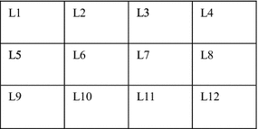

  

  Rectangular configurations

• 9. The data on number of machines, number of periods, machine sequence, present value of part movement cost, transfer batch size, distance between machine locations, money interest rate for each period (year), present value of machine rearrangement cost, the expected value, variance, and covariance of part demands in each period are known as inputs of the model.

3.2 Parameters and Indexes

The parameters and indexes used in this model are shown in Table 2.

Table 2 Notations of the proposed model

3.3 Proposed Model

In the robust layout design method, a dynamic (multi-period) layout problem is converted to a static (single period) problem. Therefore, according to the assumptions (1) and (2), the following 0-1 integer programming form of the quadratic assignment problem (QAP) formulation suggested by KOOPMANS, et al [27] is used to develop the robust machine layout design model for the SDFLP:

$$Minimize\,\sum\limits_{i = 1}^{M} {\sum\limits_{j = 1}^{M} {\sum\limits_{l = 1}^{M} {\sum\limits_{q = 1}^{M} {f_{ij} d_{lq} x_{il} x_{jq} } } } }$$

(1)

$$\begin{aligned} Subject\;to: \hfill \\ \sum\limits_{i = 1}^{M} {x_{il} ;\;\forall l} \hfill \\ \end{aligned}$$

(2)

$$\sum\limits_{l = 1}^{M} {x_{il} ;\;\forall i}$$

(3)

$$x_{il} = \left\{ \begin{array}{l} 1 \;{\text{if}}\;{\text{facility}}\;i\;{\text{is}}\;{\text{assigned}}\;{\text{to}}\;{\text{location}}\;l \hfill \\ 0\;{\text{otherwise}} \hfill \\ \end{array} \right.$$

(4)

The objective function Eq. (1) is a quadratic function of the decision variables. In this equation, $f_{ij}$ denotes the flow of materials between facilities i and j. The distance between locations l and q is denoted by $d_{lq}$. In fact, the objective function represents the total MHC, which is calculated as the summation of the product of materials flow between facilities and distance between the locations of these facilities. The linear constraints (2) and (3) ensure that each location must contain only one facility and each facility must be assigned to exactly one location respectively. Eq. (4) represents the 0-1 integer decision variables that are the solutions of the problem so that they determine the location of each facility. The robust layout for this multi-period machine layout problem is designed in such a way that the average flow of each part in different periods is considered as the part flow for the entire time planning horizon. The flow of materials for part k between machines i and j in period $t\left( {f_{tijk} } \right)$ can be calculated by using Eq. (5), where the condition $\left| {N_{ki} \text{ - }N_{kj} } \right| = 1$ refers to two consecutive operations, which are done on part k by machines i and j. The flow of part k between machines i and j over the time planning horizon $\left( {f_{ijk} } \right)$ is given in Eq. (6), which is reformed as Eq. (7) by combining with Eq. (5). According to Eq. (5), in Eq. (7) and the subsequent equations resulting from this equation, the condition $\left| {N_{ki} - N_{kj} } \right|{ = }1$ should be considered. The total flow between machines i and j resulting from all parts $\left( {f_{ij} } \right)$ is calculated by Eq. (8), which is written as Eq. (9), after combining with Eq. (7). In Eq. (9), $D_{tk}$ is a normally distributed random variable with the expected value $E\left( {D_{tk} } \right)$ and variance $Var\left( {D_{tk} } \right)$. Therefore, $f_{ij}$ is a normally distributed random variable with the expected value and variance given in Eqs. (10) and (11) respectively.

$$f_{tijk} = \left\{ {\begin{array}{*{20}c} {\frac{{D_{tk} }}{{B_{k} }}C_{tk} } & {{\text{if}}\quad \left| {N_{ki} - N_{kj} } \right| = 1} \\ 0 & {\text{otherwise}} \\ \end{array} } \right.$$

(5)

$$f_{ijk} = \frac{{\sum\limits_{t = 1}^{T} {f_{tijk} } }}{T}$$

(6)

$$f_{ijk} = \frac{1}{T}\sum\limits_{t = 1}^{T} {\frac{{C_{tk} }}{{B_{k} }}D_{tk} }$$

(7)

$$f_{ij} = \sum\limits_{k = 1}^{K} {f_{ijk} }$$

(8)

$$f_{ij} = \sum\limits_{t = 1}^{T} {\sum\limits_{k = 1}^{K} {\frac{{C_{tk} }}{{T \cdot B_{k} }}D_{tk} } }$$

(9)

$$E(f_{ij} ) = \sum\limits_{t = 1}^{T} {\sum\limits_{k = 1}^{K} {\frac{{C_{tk} }}{{T \cdot B_{k} }}E\left( {D_{tk} } \right)} }$$

(10)

$$Var(f_{ij} ) = \sum\limits_{t = 1}^{T} {\left( {\sum\limits_{k = 1}^{K} {\left( {\frac{{C_{tk} }}{{T \cdot B_{k} }}} \right)^{2} } Var(D_{tk} ) + 2\sum\limits_{k = 1}^{K} {\sum\limits_{k^{{\prime}} = k+1}^{K} {\frac{{C_{tk} \cdot C_{{tk^{{\prime }} }} }}{{T^2 \cdot B_{k} \cdot B_{{k^{{\prime }} }} }}cov(D_{tk} ,D_{tk^{{\prime}}} )} } } \right)} \,$$

(11)

In Eq. (1), considering the flow of parts as a normally distributed random variable causes the total MHC of the robust layout π _rm (i.e., $C\left( {\pi_{rm} } \right)$) to be a normally distributed random variable as well [28]. The expected value and variance of $C\left( {\pi_{rm} } \right)$ are given in Eqs. (12) and (13), respectively. Since we consider time value of money, $C_{tk}$ can be calculated using Eq. (14). For a given robust machine layout $\pi_{rm}$ if the decision maker considers $U\left( {\pi_{rm} ,p} \right)$ as the maximum value (upper bound) of $C\left( {\pi_{rm} } \right)$ with the confidence level p, then $U\left( {\pi_{rm} ,p} \right)$ given in Eq. (15) can be minimized instead of minimizing $C\left( {\pi_{rm} } \right)$ [29–31].

$$E\left( {C\left( {\pi_{rm} } \right)} \right) = \sum\limits_{i = 1}^{M} {\sum\limits_{j = 1}^{M} {E(f_{ij} )} } \sum\limits_{l = 1}^{M} {\sum\limits_{q = 1}^{M} {d_{lq} x_{il} x_{jq} } }$$

(12)

$$Var\,\left( {C\left( {\pi_{rm} } \right)} \right) = \sum\limits_{i = 1}^{M} {\sum\limits_{j = 1}^{M} {Var(f_{ij} )} } \left( {\sum\limits_{l = 1}^{M} {\sum\limits_{q = 1}^{M} {d_{lq} x_{il} x_{jq} } } } \right)^{2}$$

(13)

$$C_{tk} = C_{k} (1 + I_{r} )^{t}$$

(14)

$$U(\pi ,p) = E(C(\pi )) + Z_{p} \sqrt {Var(C(\pi ))}$$

(15)

Using Eqs. (10)-(15) the mathematical model for obtaining the robust machine layout π _rm in the SDFLP can be written as the following:

$$\begin{aligned} & Minimization\;of \hfill \\ & OFV_{rm} = \left[ {\begin{array}{l} {\sum\limits_{i = 1}^{M} {\sum\limits_{j = 1}^{M} {\sum\limits_{k = 1}^{K} {\sum\limits_{t = 1}^{T} {\frac{{C_{k} (1 + I_{r} )^{t} }}{{T.B_{k} }}} E(D_{tk} )\sum\limits_{l = 1}^{M} {\sum\limits_{q = 1}^{M} {d_{lq} x_{il} x_{jq} } } } } } } \\ { + Z_{p} \left( {\sum\limits_{i = 1}^{M} {\left( {\sum\limits_{j = 1}^{M} {\left( {\sum\limits_{t = 1}^{T} {\begin{array}{l} {\sum\limits_{k = 1}^{K} {\left( {\frac{{C_{k} (1 + I_{r} )^{t} }}{{T.B_{k} }}} \right)^2Var(D_{tk} ) + } } \\ {2\sum\limits_{k = 1}^{K} {\sum\limits_{{k^{{\prime }} = k + 1}}^{K} {\frac{{C_{k} .C_{k^{{\prime}}} (1 + I_{r} )^{2t} }}{{T^2.B_{k} .B_{{k^{{\prime }} }} }}\text{cov} (D_{tk} ,D_{{tk^{{\prime }} }} )} } } \\ \end{array} } } \right)} } \right)\left( {\sum\limits_{l = 1}^{M} {\sum\limits_{q = 1}^{M} {d_{lq} x_{il} x_{jq} } } } \right)}^{2} } \right)^{{{1 \mathord{\left/ {\vphantom {1 2}} \right. \kern-0pt} 2}}} } \\ \end{array} } \right] \hfill \\ \end{aligned}$$

(16)

Subject to: Eqs. (2)-(4).

Eq. (16) symbolized by OFV _rm denotes the objective function (also termed cost function) of the robust machine layout design model. In this model, all parameters, which are defined in Table 2, are known in advance. In fact, this model is deterministic, although part demands, which have the known expected value and variance in each period, are random variables. However, the optimal values of the unknown 0-1 integer decision variables $x_{il}$ are obtained by solving the model. The optimal location of each machine is thus determined and in turn, the robust machine layout π _rm is obtained throughout the time planning horizon.

4 Verification and Validation of the Proposed Model

This section aims to verify and validate the proposed model using numerical examples (i.e., to generate a large number of test problems at random), benchmark (data from literature), real case studies, and sensitivity analysis methods. The effect of assuming dependent part demands and time value of money (interest rate) on total cost of the proposed model is also investigated. Rectangular layout configuration is considered by computing rectilinear distance between centers of machines. Dynamic programming (DP) method is used for solving the randomly generated and benchmark problems discussed in sections 4.1 and 4.2 respectively. This is done because DP is an exact method to find the optimal solution of the problems. Therefore, the model validation and analysis carried out in the two aforementioned sections will be more secure than the meta-heuristic approaches such as simulated annealing (SA) algorithm used to solve the problems. It is essential to note that the obtained solution using meta-heuristics is not necessarily an optimal solution, particularly for large-sized problems. However, the real case study is solved using the SA algorithm due to the size of the problem because DP cannot solve it in a reasonable time. This algorithm is coded in MATLAB and run using a PC with an Intel 2.10 GHz CPU and 3 GB RAM.

4.1 Numerical Examples

To validate the proposed model, 104 different-sized randomly generated test problems with $2\text{ < }M\text{ < }9$ and $1\text{ < }T\text{ < }7$ are applied to the proposed model. The test problems are also solved in accordance with the static layout design approach. By doing so, for each model, 104 cost function values, which are considered as samples of a population, are obtained.

As we know from statistics, the $100*\left( {1 - \alpha } \right)\%$ confidence interval for difference between means of two populations is calculated as Eq. (17), where $n_{1}$ and $n_{2}$ are sample size, $\overline{x}_{1}$ and $\overline{x}_{2}$ are sample means, $\sigma_{1}^{2}$ and $\sigma_{2}^{2}$ are sample variances, and $z_{\alpha /2}$ is standard normal Z value so that ${ \Pr }\left( { - z_{\alpha /2} \le Z \le z_{\alpha /2} } \right) = 1 - \alpha$. The sample mean and sample variance are given in Eqs. (18) and (19) respectively.

$$(\overline{x}_{1} - \overline{x}_{2} ) - z_{\alpha /2} \sqrt {\frac{{\sigma_{1}^{2} }}{{n_{1} }} + \frac{{\sigma_{2}^{2} }}{{n_{2} }}} < \mu_{1} - \mu_{2} < (\overline{x}_{1} - \overline{x}_{2} ) + z_{\alpha /2} \sqrt {\frac{{\sigma_{1}^{2} }}{{n_{1} }} + \frac{{\sigma_{2}^{2} }}{{n_{2} }}}$$

(17)

$$\overline{x} = \frac{{\sum\limits_{i = 1}^{n} x_{i} }}{n}$$

(18)

$$\sigma^{2} = \frac{1}{n - 1}\sum\limits_{i = 1}^{n} {\left( {x_{i} - \overline{x} } \right)^{2} }$$

(19)

Using Eq. (17), the 95% confidence intervals for the difference between the populations are calculated as follows: $- 14250 \, < \mu_{r} - \mu_{s} < \, 15840$, where μ _r and μ _s are the mean value of the cost function of the robust model and the static model, respectively.

As we know, the static approach generates an optimal layout for each period. Therefore, it is used as a benchmark to evaluate the performance of the robust layout. The obtained confidence interval is almost a symmetric interval. Thereby, the cost function values of each period for the robust and static layouts are near to each other. To illustrate the conclusion, a numerical example is constructed by using a test problem taken from BALAKRISHNAN, et al [32] in such a way that the flow matrix is considered as the matrix of expectation of flow denoted by E. The matrix of variance of flow denoted by V is computed by $V = E/3$. Additional input data of this problem are as follows: it includes six facilities and five periods. As mentioned, rectangular layout configuration is considered by computing rectilinear distance between centers of machines. This problem is applied to the robust and static models by considering a 0.75 percentile level. Finally, the numerical example is solved using DP algorithm and the results are shown in Table 3.

Table 3 Results of the example for robust, and static models

As mentioned in Section 1, the static and robust approaches are suitable for facility layout design in the cases of low and high rearrangement costs, respectively. It is difficult to relate MHCs with rearrangement costs. However, we assume that the aforementioned conditions for rearrangement costs allowing us to use the static and robust approaches are met in advance. In fact, since neither the static model nor the robust model consider the facility rearrangement cost value, there is no need to mention them here. In the static approach, each period is solved separately regardless of data from other periods as well as ignoring the low rearrangement cost. Using this approach an optimal layout, which can be easily changed from period to period, is obtained for each period. On the other hand, using the proposed robust layout design model with the objective function given in Eq. (16), only grants one layout for the entire time planning horizon. As shown in Table 3, each of the five periods has different layouts using the static approach. However, the robust layout [564123] is obtained for the whole time planning horizon by using the robust model.

Thereby, the static layout suffers from the rearrangement cost from period to period, while the robust layout is free of this cost. To evaluate the behavior of the robust layout [564123], which is fixed throughout the planning horizon, we calculate its MHC in each period and in the entire planning horizon. Then, the MHC of the layouts obtained by the static approach is also computed for each period and throughout the planning horizon. As mentioned, the static approach generates an optimal layout for each period, and thereby it can be used as a benchmark for evaluating the performance of the proposed robust layout. The MHC of each period for static and robust approaches is compared with each other in Fig. 2. On comparison, in each period, the MHC of the robust layout is larger than that of the static layout. Therefore, the robust layout is not necessarily an optimal layout for each period. The results also show that in most periods, the MHC of the robust layout is close to that of the static layout, which is the optimal value. In addition, considering the whole time planning horizon, the difference between the total costs of the robust layout (132582) and the static one (122505) is 7.6%. The MHC results in most periods for random demands, however, are relatively close to the optimal value of the static layout, as shown in Fig. 2. Over the entire planning horizon, the difference between the total costs of the robust layout (132582) and the static one (122505) is 7.6%, making the robust layout reasonably efficient for the whole time planning given the randomly varying demands now.

Fig. 2

Total cost of static and robust layouts in each period

4.2 Benchmark Study

Since there is no historical data on the expectation and variance of demands in each period, the proposed model is tested in a deterministic environment by comparing it with the previous approaches as benchmark data. To this end, a 50% percentile level (p = 50%) equivalent of z _p  = 0 is applied to the model. By doing so, the second term of the objective function given in Eq. (16) containing variance of parts demand is ignored. This also implies that the data on the variance of the part demands in each period are not required. Hence, the demand of parts in each period, which is known in the deterministic case, is regarded as the expectation of parts demand in the proposed model. For simplicity and without losing the generality of the proposed model, independent product demands are considered, and thereby there is no correlation between demands. As a result, in Eq. (16), the term covariance is zero. The data set used for testing the proposed model is taken from YAMAN, et al [33]. The input data are as follows: The problem includes nine machines and five periods. Data on machine sequence and part demand in different periods are given in Tables 4 and 5, respectively. Rectangular layout configuration is considered so that location grid of 3 × 3 is used as facilities locations. Part movement cost, and batch size are set to ten and one, respectively.

Table 4 Data on machine sequence

Table 5 Part demand in different periods

As mentioned, MADHUSUDANAN-PILLAI, et al [6]. proposed an SA algorithm to solve their robust layout design model, which is termed MP-SA hereafter. Another heuristic method was developed by IRAPPA-BASAPPA, et al [5]. to solve their model, which is denoted by I-M hereafter.

YAMAN, et al’s [33] problem is applied to the proposed robust machine layout model. To calculate the MHC of each period, the obtained robust layout is applied to the demands data in different periods of the planning horizon. Table 6 shows the results of the proposed robust layout design model and the previous methods. On comparison, the proposed model has the best performance with respect to the I-M and MP-SA methods in each period. In addition, the proposed robust model can be applied to both deterministic and stochastic environments, whereas the model developed by IRAPPA-BASAPPA, et al [5] can only be used for deterministic environment. Table 7 shows the total MHC over the entire planning horizon obtained by the proposed robust model and the previous approaches including the MAIN method suggested by CHAN, et al [34], the I-M, and MP-SA methods. Based on the various results, the proposed robust model has the best performance so that it leads to 2.7% improvement in total cost with respect to MP-SA method, which is the best previous method. It is necessary to mention that in this section, to validate the proposed robust model only one test problem taken from the literature is solved. Therefore, unlike the approaches done in section 4.1, there is no need to state the significant level for the 2.7% improvement in total cost. Tables 6 and 7 are examples of using our proposed model in the deterministic case.

Table 6 MHC of the robust model and previous approaches

Table 7 Total MHC of the robust model and previous approaches

Facility layout design application example

According to KRISHNAN, et al [35], in the real world case study, six parts are processed using 21 equal-sized machines $\left( {35^{{\prime }} \times 35^{{\prime }} } \right).$ Part movement cost and machine rearrangement cost are presumed to be $3.75/foot and zero respectively. An aisle space of 10 feet is assumed to be considered around each machine. Euclidean distance between centers of machines is considered in the case study. The data on yearly part demands, which are given in Table 8, are considered as the expectation of the part demands. Since there is no data on variance of part demands, a 50% percentile p equivalent of z _p  = 0 is considered. Machine sequence data are given in Table 9. The data of the problem are applied to the proposed robust machine layout design model and is solved using an SA algorithm. SA is an intelligent approach that has been widely used to solve the FLP. It is a simulation of physical annealing process of solids in statistical mechanics, which starts with a known or randomly generated initial solution and a high initial value of temperature. It is formed by two loops, namely, the inner loop to search for a neighboring solution, and the outer loop for decreasing the temperature to reduce the probability of accepting the non-improving neighboring solutions in the inner loop. Table 10 shows the results of our method and that of the best previous one including the cost associated with each period and the total cost over the whole time planning horizon. As shown in Table 10, the obtained robust machine layout leads to 7.35% improvement with respect to the best previous one proposed by KRISHNAN, et al [35]. Using the same reason as in previous section, there is no need to state the significant level for the 7.35% improvement.

Table 8 Expectation of part demands for real case study

Table 9 Machine sequence for real case study

Table 10 Results of real case study

4.3 Sensitivity Analysis

In this section, sensitivity analysis is performed for validating the proposed model and to rank the inputs of the model in terms of the degree of their impact on the output of the model (objective function). Sensitivity of the output of the proposed robust machine layout design model with respect to the input parameters including expectation of materials flow, variance of materials flow, and confidence level is investigated by using one-way analysis of variance (ANOVA). Using this technique, the null and alternative hypotheses are usually tested by using the F-test. The null hypothesis states that the means amongst two or more groups are equal and the alternative one indicates that at least two means are different. In ANOVA, it is assumed that the mean of the model outputs for each group is normally distributed random variable with approximately the same variance. Considering the assumptions, the F-value is statistically important at $p < 5\%$ and the null hypothesis is rejected [36]. In ANOVA, an input and an output of a model are referred to as a “factor” and a “response variable” respectively [37]. The factors are ranked according to the F-values [38]. Inputs with higher F-values are more sensitive factors, which more strongly affect the output of a model. The aim of one-way ANOVA is to realize whether data from several groups have the same mean.

To perform the sensitivity analysis, 100 randomly generated test problems are applied to the proposed model in three different cases, namely, Cases E, V, and P, which investigate the sensitivity of the objective function of the model with respect to expectation of materials flow (matrix E), variance of materials flow (matrix V) and confidence (percentile) level (p) respectively. The input data are as follows: For each test problem, the expectation and variance of part demands (E and V) are randomly generated with uniform distribution so that $E \in (1000,10000)$ and $V \in (1000,3000)$. Besides, the number of machines and the number of periods are six and three respectively $\left( {M = { 6},T = 3} \right)$.

In Case E, matrix E is changed by $E^{{\prime }} = E + r*E$, whereas matrix V and confidence level p remain unchanged. Considering nine different values of $r \in A = \left\{ {01, 0.2, 0.3, 0.4, 0.5, 0.6, 0.7, 0.8, 0.9} \right\}$ leads to generate nine different matrices E. Each test problem is solved for each of the nine different Es so that the optimal value of each objective function corresponds to each E is obtained. Similarly, in Case V, matrix V is changed by $V^{{\prime }} = V + r*V$,whereas matrix E and confidence level p remain unchanged. Considering the nine aforementioned values of r leads to generate nine different matrices V. Each test problem is solved for each of the nine different V so that the optimal value of each objective function corresponding to each V is obtained. Finally, in Case P, the confidence level p is set to each element in A while matrices E and V remain unchanged. Similar to the two former cases, each test problem is solved for each of the nine different p values so that the optimal value of each objective function corresponding to each p is obtained. In fact, each case includes nine groups (populations) and each group contains 100 samples of objective function values. Each case, group, and sample is denoted by k, g, and s, respectively, where $\left( {k = {\text{ E}},{\text{ V}},{\text{ P}}} \right), \, \left( {{\text{g}} = \, 1, \, 2, \ldots ,9} \right)$, and $\left( {s = { 1},{ 2}, \ldots ,{ 1}00} \right)$. Mean of samples within group g in case k is represented by $\mu_{g}^{k}$. As mentioned, the condition of having normal distribution for the mean of each group is necessary for ANOVA. To meet this condition, 100 randomly generated test problems are considered. This is due to the central limit theorem (CLT), which states that the average of a sufficiently large number (for example, $\ge 30)$ of independent random variables follows normal distribution [39].

The aim of this section is to test the hypothesis given in Table 11 using ANOVA. Using MATLAB software, ANOVA is applied to the results of the randomly generated test problems for testing the aforementioned hypothesis. The results of ANOVA are given in Table 12. According to the results including F-values and P-values, the null hypothesis H ₀ is rejected. In other words, as expected, different values of input parameters containing expectation of product demands, variance of product demands, and confidence level lead to designing different facility layout. Therefore, the model validation concludes. As mentioned, the input with higher F-value is the more sensitive parameter. According to F-values in Table 12, the expectation of product demand and the variance of product demand are the most and least sensitive parameters, respectively. This is because of $\left( {F_{E} = 7.98} \right) > \left( {F_{P} = 3.05} \right) > \left( {F_{V} = 0.37} \right)$, where $F_{E} ,F_{V}$, and $F_{p}$ are F- values in the Cases E, V, and P respectively. Experimentally, we concluded that changes in the parameters including number of machines, number of periods, confidence level, and the range in which the expectation and variance of product demands are randomly generated can change the sensitivity ranking of the inputs studied in this section.

Table 11 Hypotheses needed for sensitivity analysis using ANOVA

Table 12 Results of ANOVA (SS means sums of squares; df means degrees of freedom; MS means mean squares; F = SS/df)

5 Demands Correlation and Interest Rate Affects Total Cost

In this section, the effect of assuming dependent part demands and time value of money (interest rate) on total cost of the proposed model is investigated. To this end, a numerical example with input data given in Table 13 is applied to the model. For the known solution, the values of objective function of the proposed model is calculated by considering different p percentile levels in the three following cases: (i) independent demands with no interest rate, (ii) dependent demands with no interest rate, and (iii) independent demands with non-zero interest rate. The results are shown in Table 14.

Table 13 Example for analyzing demands correlation and interest rate

Table 14 Total cost for three cases

Using the results, the curve of the total cost with respect to confidence level is plotted in Fig. 3. The figure indicates that non-zero interest rate leads to increased total cost over the range of uncertainty. As shown in the figure, the cost function has the same value for $p = 0.5$ for both independent and dependent demands, because this percentile level, which is equivalent of $z_{p} = \, 0$, leads to ignoring the second term of the objective function of the proposed model given in Eq. (16). According to the equation, the second term of the objective functions is variance of MHC, which is function of demands correlation indicated by covariance. Therefore, by ignoring this term, demands correlation does not affect the total cost. In other words, if the user-defined percentile level is 0.5, independency or dependency of demands does not affect the total cost. It is necessary to state that in Eq. (16), for independent and dependent demands, the term of covariance is zero and non-zero respectively. Besides, the total cost is decreased for $p < 0.5$ (equivalent of $z_{p} < \, 0$) and increased for $p > 0.5$ (equivalent of $z_{p} > \, 0$) percentile levels by considering dependent demands.

Fig. 3

Demands correlation and time value of money

6 Conclusions

In this paper, a novel QAP-based mathematical model was proposed for design of a robust machine layout for the SDFLP. The proposed model was validated by using numerical examples, benchmarks, and sensitivity analysis methods. The effect of assuming dependent part demands and interest rate on total cost of the proposed model was investigated. According to the findings, the following conclusions were obtained: (i) The robust layout is a good layout for all periods in the planning horizon, although it is not necessarily an optimal layout for each period. (ii) According to the cost values in each period and the total cost value in the planning horizon, the robust layout obtained by solving the proposed model, has the best performance with respect to the previous models in literature. (iii) The proposed robust model can be applied to both deterministic and stochastic environments, whereas the previous models can only be used for deterministic environments. The Raytheon Aircraft Company studied by KRISHNAN, et al [34] was a real world FLP including 21 equal-sized machines that was solve by our proposed model. On the basis of findings, the obtained robust machine layout leads to 7.35% improvement with respect to the best previous one proposed by KRISHNAN, et al [34]. (iv) Sensitivity analysis indicated that different values of input parameters containing expectation of product demands, variance of product demands, and confidence level lead to design of different facility layout. Besides, the expectation of product demand and the variance of product demand are the most sensitive and the least sensitive parameters, respectively. However, changes in the parameters including number of machines, number of periods, confidence level, and the range in which the expectation and variance of product demands are randomly generated can change the sensitivity of the inputs. (v) Considering nonzero interest rate leads to increased total cost over the range of uncertainty. (vi) The total cost is decreased for $p < 0.5$ (equivalent of $z_{p} < \, 0$) and increased for $p > 0.5$ (equivalent of $z_{p} > \, 0$) by considering dependent demands. Besides, the numerical examples solved in Sections 4.3 and 5 indicate that the proposed model is applicable to stochastic environment.

7 Limitation and Future Works

Since the proposed model was developed based on the QAP formulation, it can be applied to any manufacturing systems, particularly the modern ones such as cellular manufacturing systems (CMS) and flexible manufacturing systems (FMS) with equal-sized facilities. The assumption of equal-sized facilities can be regarded as a restriction or a weakness. However, it can be justified as follows: in practice, there are some manufacturing systems such as the real case mentioned in Section 4.2 and the Vought Aerospace Company in Dallas, Texas [3] with equal-sized facilities.

As another subjective limitation, the same machining time on each machine may also be deduced from the assumption of equal-sized machines, which seem to be identical. Conversely, the equal-sized machines can be multi-functional machines such as the ones used in FMSs. Considering so, the machining time on each machine is not necessary the same and depends on the process done by machine in accordance with production process. According to GROOVER [3], some real world examples of the FMSs established in the United States of America are as follows: Vought Aerospace in Dallas, Texas; Flexible Fabricating systems for automated sheet-metal processing; IngersollRand Company in Roanoke, Virginia; Assembly FMS installed by Allen-Bradley Company; John Deer American Corporation that manufactures agricultural machines; General Electric Company; and Caterpillar Tractor.

If the production horizon increases, such as 12 months × 5 years, the number of variables in the problem formulation will sharply increase and, as expected, the computational time will increase and/or the SA algorithm may yield a poor solution quality. It is also essential to mention that since the SA algorithm is a randomly local search technique, it can solve the large-sized problems in a reasonable computational time so that a sub-optimal solution can be obtained.

In this study, alternate process plans have not been considered. Considering alternate process plans leads to increasing the complexity of the proposed models and in turn to increasing the computational time. Some other constraints and issues such as unequal-sized machines/cells, adding and removing machines in different periods, closeness ratio, aisles, budget constraint for total cost, machine reliability and deadlock problem can be considered in future studies.

References

TOMPKINS J A, WHITE J A, BOZER Y A, TANCHOCO J M A. Facilities planning[M]. New York: Wiley, 2003.
BALAKRISHNAN J, CHENG C H. multi-period planning and uncertainty issues in cellular manufacturing: a review and future directions[J]. European Journal of Operational Research, 2007, 177: 281–309.
GROOVERMP. Automation, production systems, and computer-integrated manufacturing[M]. 4th ed. New Jersey: Pearson Education Inc., 2016.
MOSLEMIPOUR G, LEE T S, RILLING D. A review of intelligent approaches for designing dynamic and robust layouts in flexible manufacturing systems[J]. Int. J. Advanced Manuf. Tech., 2012, 60: 11–27.
IRAPPA-BASAPPA H, MADHUSUDANAN-PILLAI V. Development of a heuristic for layout formation and design of robust layout under dynamic demand[C]//Proceedings of the International Conference on Digital Factory ICDF, August 11–13, 2008: 1398–1405.
MADHUSUDANAN-PILLAI V, IRAPPA-BASAPPA H, KRISHNA K K. Design of robust layout for dynamic plant layout problems[J]. Computers & Industrial Engineering, 2011, 61: 813–823.
SOOLAKI M, IZADI A. A robust optimisation model for manufacturing cell design problem under uncertainty[J]. International Journal of Services and Operations Management, 2013, 15(2): 238–258.
FORGHANI K, MOHAMMADI M, GHEZAVATI V. Designing robust layout in cellular manufacturing systems with uncertain demands[J]. International Journal of Industrial Engineering Computations, 2013, 4(2): 215–226.
NEGHABI H, ESHGHI K, SALMANI M H. A new model for robust facility layout problem[J]. Information Sciences, 2014, 278: 498–509.
NEMATIAN J. A robust single row facility layout problem with fuzzy random variables[J]. Int. J. Adv. Manuf. Technol., 2014, 72: 255–267.
POURVAZIRI H, NADERIB B. A hybrid multi-population genetic algorithm for the dynamic facility layout problem[J]. Applied Soft Computing, 2014, 24: 457–469.
AZADEH S, HAGHIGHI S M, ASADZADEH S M. A novel algorithm for layout optimization of injection process with random demands and sequence dependent setup times[J]. Journal of Manufacturing Systems, 2014, 33: 287–302.
FAZLELAHI F Z, POURNADER M, GHARAKHANI M, et al. A robust approach to design a single facility layout plan in dynamic manufacturing environments using a permutation-based genetic algorithm[J]. Proc IMechE Part B:J Engineering Manufacture, 2015, DOI: 10.1177/0954405415615728.
DERAKHSHAN ASL A, KUAN K Y. Solving unequal-area static and dynamic facility layout problems using modified particle swarm optimization[J]. J. Intell. Manuf., 2015, DOI: 10.1007/s10845-015-1053-5.
SEE P C, WONG K Y. Application of ant colony optimisation algorithms in solving facility layout problems formulated as quadratic assignment problems: a review[J]. Int. J. Industrial and Systems Engineering, 2008, 3(6): 644–672.
LEE HY, KANG S, CHAE J. Mutation effects in a genetic algorithm for a facility layout problem in QAP form[J]. International Journal of Advanced Logistics, 2015, 4(3): 170–179.
KULTUREL-KONAK S, SMITH A E, NORMAN B A. Layout optimization considering production uncertainty and routing flexibility[J]. International Journal of Production Research, 2004, 42(21): 4475–4493.
ZHAO Y, WALLACE S W. Integrated facility layout design and flow assignment problem under uncertainty. INFORMS Journal on Computing, 2014, 26(4): 798–808.
RIPON KS N, GLETTE K, HOVIN M, et al. Dynamic facility layout problem under uncertainty: a Pareto-optimality based multi-objective evolutionary approach[J]. Cent. Eur. J. Comp. Sci, 2011, 1(4): 375–386.
ARIAFAR S, ISMAIL N, TANG S H, et al. A stochastic facility layout model in cellular manufacturing systems[J]. International Journal of the Physical Sciences, 2011, 6(15): 3666–3670.
SHUMSKY ZHANG. Dynamic capacity management with substitution[J]. Operations Research, 2009, 57(3): 671–684.
KRISHNAN K K, CHERAGHI S H, NAYAK C N. Facility layout design for multiple production scenarios in a dynamic environment[J]. Int. J. Industrial and Systems Engineering, 2008, 3(2): 105–133.
TAHA Z, ROSTAM S. A fuzzy AHP–ANN-based decision support system for machine tool selection in a flexible manufacturing cell[J]. Int. J. Adv. Manuf. Technol., 2011, 57: 719–733.
WANG J, LI J, ARINEZ J, et al. Quality analysis in flexible manufacturing systems with batch productions: performance evaluation and nonmonotonic properties[J]. IEEE Transaction on Automation Science and Engineering, 2010, 7(3): 671–676.
CHEN H, WANG A, NING R, et al. Layout planning technology of cellular manufacturing system based on process interconnection analysis[J]. Chinese Journal of Mechanical Engineering, 2011, 24(6): 1035–1044.
LEI D, WU Z. Integration of cell formation and layout design in the unidirectional loop material handling environment[J]. Chinese Journal of Mechanical Engineering, 2005, 18(2): 286–289.
KOOPMANS T C, BECKMAN M. Assignment problems and the location of economic activities[J]. Econometric, 1957, 25: 53–76.
BRAGLIA M, SIMONE Z, ZAVANELLA L. Layout design in dynamic environments: Analytical issues[J]. International Transactions in Operational Research, 2005, 12: 1–19.
MOSLEMIPOUR G, LEE T S. Intelligent design of a dynamic machine layout in uncertain environment of flexible manufacturing systems[J]. J. Intell. Manuf., 2012, 23: 1849–1860.
NORMAN B A, SMITH A E. A continuous approach to considering uncertainty in facility design[J]. Computers and Operations Research, 2006, 33: 1760–1775.
BALAKRISHNAN J, CHENG C H. Genetic search and the dynamic layout problem[J]. Computers and Operations Research, 2000, 27(6): 587–593.
YAMAN A, GETHIN D T, CLARKE M J. An effective sorting method for facility layout construction[J]. International Journal of Production Research, 1993, 31(2): 413–427.
CHAN W M, CHAN C Y, KWONG C K. Development of the MAIN algorithm for a cellular manufacturing machine layout[J]. International Journal of Production Research, 2004, 42(1): 51–65.
KRISHNAN K K, CHERAGHI SH, NAYAK C N. Dynamic from-between chart: a new tool for solving dynamic facility layout problems[J]. Int. J. Industrial and Systems Engineering, 2006, 1(1/2): 182–200.
SHARMA S. Applied multivariate techniques[M]. New York: John Wiley & Sons, Inc., 1996.
NETER J, KUTNER MH, NACHTSHEIM C J. Applied linear statistical models[M]. 4th ed. Chicago, IL, USA: McGraw-Hill, 1996.
CARLUCCI A, NAPOLITANO F, GIROLAMIA, et al. Methodological approach to evaluate the effects of age at slaughter and storage temperature and time on sensory profile of lamb meat[J]. Meat Science, 1999, 52(4): 391–395.
LEDOLTER J, HOGG R. Applied statistics for engineers and physical scientists[M]. 3rd ed. New Jersey: Pearson Education Inc., 2010.
Author information
Authors and Affiliations
Corresponding author
Additional information
Supported by the Ministry of Higher Education of Malaysia through the Foundation Research (Grant Scheme no. FRGS/1/2012/TK01/MMU/02/2).
Rights and permissions
About this article
Cite this article
MOSLEMIPOUR, G., LEE, T.S. & LOONG, Y.T. Performance Analysis of Intelligent Robust Facility Layout Design. Chin. J. Mech. Eng. 30, 407–418 (2017). https://doi.org/10.1007/s10033-017-0073-9
Received:
Revised:
Accepted:
Published:
Issue Date:
DOI: https://doi.org/10.1007/s10033-017-0073-9