- Original Article
- Open access
- Published:
DADOS: A Cloud-based Data-driven Design Optimization System
Chinese Journal of Mechanical Engineering volume 36, Article number: 34 (2023)
Abstract
This paper presents a cloud-based data-driven design optimization system, named DADOS, to help engineers and researchers improve a design or product easily and efficiently. DADOS has nearly 30 key algorithms, including the design of experiments, surrogate models, model validation and selection, prediction, optimization, and sensitivity analysis. Moreover, it also includes an exclusive ensemble surrogate modeling technique, the extended hybrid adaptive function, which can make use of the advantages of each surrogate and eliminate the effort of selecting the appropriate individual surrogate. To improve ease of use, DADOS provides a user-friendly graphical user interface and employed flow-based programming so that users can conduct design optimization just by dragging, dropping, and connecting algorithm blocks into a workflow instead of writing massive code. In addition, DADOS allows users to visualize the results to gain more insights into the design problems, allows multi-person collaborating on a project at the same time, and supports multi-disciplinary optimization. This paper also details the architecture and the user interface of DADOS. Two examples were employed to demonstrate how to use DADOS to conduct data-driven design optimization. Since DADOS is a cloud-based system, anyone can access DADOS at www.dados.com.cn using their web browser without the need for installation or powerful hardware.
1 Introduction
Most engineering design optimization problems require experiments and/or numerical simulations to evaluate design objectives and constraints as a function of design variables [1]. For many practical engineering applications, however, it can take hours, or even days to conduct a single simulation. As a result, routine tasks such as design space exploration, design optimization, and sensitivity analysis tend to be impossible since they require thousands of simulation evaluations, let alone the experiments.
Data-driven design optimization can alleviate this burden significantly by constructing inexpensive approximation models to replace the time-consuming simulations and costly experiments. Terminologically, data-driven design optimization is an engineering design methodology using data science algorithms to create approximation models, also known as surrogate models, to facilitate quick exploration of design alternatives and obtain the optimal design [2]. Surrogate models [3, 4] are constructed using a data-driven approach. The exact inner working of the simulation code or the mechanism of the experiment is not necessary to be known or even understood, only the input-output relationship matters [5]. A surrogate model is constructed by the samples comprising a limited number of intelligently chosen data points and their corresponding outputs of the simulation or experiment. Once the surrogate model is built successfully, it can be used to predict the performance of a new design rapidly. Also, it can be coupled with sensitivity analysis to identify the impact of each design variable on the output. In addition, an optimal design can be obtained efficiently by surrogate and optimization algorithms. Data-driven design optimization is gaining popularity in various engineering fields because it can significantly reduce the computational budget, save experimental costs, and accelerate the optimization process.
To further facilitate the development and application of data-driven design optimization, software packages have been developed. The software package DACE (Design and Analysis of Computer Experiments) [6] can be regarded as the most famous early work in the field. DACE is a Matlab toolbox specialized in constructing kriging approximation models as surrogates for numerical simulations. ooDACE [7] is another Matlab toolbox focusing on the variants of kriging, including simple kriging, ordinary kriging, universal kriging, blind kriging [8], and regression kriging [9]. These two software packages have been popularized in the academic community. However, these two primarily focus on the approximation part of the data-driven design optimization, thus, the entire process of the data-driven design optimization cannot be fulfilled completely without recourse to other toolboxes. Subsequently, software packages including more functionalities are developed, for example, SURROGATE toolbox [10], SUMO [11], MATSuMoTo [12], and SMT [13]. The SURROGATE toolbox is a general-purpose library of multivariate function approximation and optimization methods for Matlab and Octave. This toolbox contains the necessary modules to perform data-driven design optimization, e.g., design of experiments (DoE), surrogates, model validation and selection, optimization, and sensitivity analysis. Most importantly, it is free, open-source software. SUMO is a Matlab toolbox having similar functionalities to the SURROGATE toolbox. Besides, it has an excellent pluggable and extensible ability so that it can be used as a common platform to test and benchmark different sampling and approximation methods while easily integrating into the engineering design process. The SUMO toolbox is available in two forms: the fully functional proprietary version for commercial use and the restricted academic version. MATSuMoTo is a surrogate global optimization toolbox for Matlab. It can solve the computationally expensive, black-box global optimization problems that may have continuous, mix-integer, or pure integer variables. SMT is a Python open-source surrogate modeling toolbox that contains a bundle of sampling methods and surrogate modeling techniques. SMT is different from the aforementioned toolboxes because it can leverage derivative information, including training derivatives used for gradient-enhanced modeling, prediction derivatives, and derivatives with respect to training data. In addition, it also includes its own in-house surrogate techniques: kriging by partial least-squares reduction, which scales well with the dimensionality of the problem; and energy-minimizing spline interpolation, which scales well with the number of training points.
It is encouraging that there are several software packages dedicated to the development and application of data-driven design optimization, however, most of the above toolboxes have gained popularity solely in academia rather than the industry. This is because the above toolboxes only employ command-line interfaces for algorithm configurations and executions, which creates a significant barrier for engineers, especially those who do not familiar with the optimization theory and programming, to use them. To address this issue, design optimization tools with a user-friendly graphical user interface (GUI) have been developed. Liu et al. developed a Matlab GUI toolbox [14] for surrogate-based design and optimization. For the sake of simplicity and easy-to-use, this toolbox only contains the most fundamental modules, e.g., DoE, surrogate model, and optimization, to help users perform design optimization. In addition, various commercial software has been developed, such as Dassault Systèmes SIMULIA’s Isight, Phoenix Integration’s ModelCenter, Esteco’s modeFrontier, DATADVANCE’s pSeven, and PIDOTECH’s PIAnO. These commercial software products can partially automate complex analysis and design procedures by integrating cross-disciplinary models and applications in a simulation process flow. Moreover, users can explore the design space and identify the optimal design parameters through a professional GUI. While these commercial software products have made it easier for users to implement analysis and design optimization, the built-in algorithms, especially the surrogate techniques used to approximate the relationship between system inputs and outputs, are usually not state-of-the-art. In addition, with the increase in versatility and functionality, the commercial software products tend to be cumbersome and steepen the learning curve for beginners.
In this work, we developed an easy-to-use cloud-based data-driven design optimization system, named DADOS. DADOS transforms the tradition of local installation and single-user operating, to cloud operating, multi-person and multi-disciplinary optimization. With DADOS, users can get the optimized performance of products easily and efficiently. DADOS has the following advantages:
-
(1)
DADOS has a library of state-of-the-art algorithms and is flexible for expanding. DADOS has nearly 30 key algorithms, including design of experiments, surrogate models, model validation and selection, prediction, optimization, and sensitivity analysis, which help users thoroughly explore design alternatives and identify the optimal performance parameters. In addition, DADOS is flexible for expanding and allows users to upload their in-house code.
-
(2)
DADOS is easy-to-use. DADOS employed flow-based programming that wraps up specific algorithms into a block and integrates these blocks into a workflow. With DADOS, users don’t need to program to conduct performance prediction, optimization, and sensitivity analysis. Just by dragging, dropping, and connecting these algorithm blocks, they can get these jobs done.
-
(3)
DADOS supports multi-person, multi-disciplinary optimization. An engineering project generally needs engineers and designers from different fields of engineering to complete. DADOS allows multi-person working on a project at the same time and supports multi-disciplinary optimization. Members in the same group have access to the work progress and details at any time because DADOS is cloud-based and the data is backed up timely.
-
(4)
With DADOS, there’s nothing to upgrade or install. DADOS is a cloud-based system, there is no need to download or install it. Just log in with a web browser, and users can access DADOS at any time, any place, and for free.
The remainder of this paper is organized as follows. Section 2 introduces the workflow of conducting data-driven design optimization. Section 3 presents the architecture and details the user interface of DADOS. In Section 4, a numerical example and a real-world engineering application are used to demonstrate how to use DADOS to conduct data-driven design optimization. Conclusions and future work are drawn in Section 5.
2 Data-driven Design Optimization
This section details the workflow of conducting data-driven design optimization and briefly introduces an exclusive hybrid surrogate technique in DADOS.
2.1 The Workflow of Data-driven Design Optimization
Data-driven design optimization is gaining popularity in various engineering fields because it can significantly reduce the computational budget, save experimental costs, and accelerate optimization process. The workflow of conducting data-driven design optimization is illustrated in Figure 1.

The workflow of conducting data-driven design optimization
2.1.1 Problem Formulation
When dealing with a design optimization problem, the first thing that needs to be done is to formulate the problem. That is, extracting the design variables and their ranges from the practical problem, and determining the quantities of interest, design objectives, and constraints.
2.1.2 Design of Experiments
After the problem formulation is finished, the initial samples are required to be generated to build the surrogate. Since each sample is corresponding to a single run of simulation or experiment, the number of samples is severely limited by the expense of each sample. As a result, how to choose samples wisely in the given design space is a key problem. This practice is known as the design of experiments. It is preferable to have samples that are distributed evenly across the design space. A sampling plan possessing this feature is called space-filling. In this way, the input-output relationship from all regions of the design space could be captured by the limited number of samples. There are many DoE techniques to determine the set of sample points, such as full factorial design (FFD) [15], orthogonal arrays (OA) [16], central composite designs (CCD) [17], Latin hypercube sampling (LHS) [18], and optimal LHS (OLHS) [19].
2.1.3 Output Evaluations
Once the initial samples of design variables have been determined, their corresponding output values should be evaluated by running simulations or experiments. Then, a dataset can be obtained by assembling the pairs of the inputs (i.e., the samples of design variables) and their corresponding outputs.
2.1.4 Construction of Surrogate Models
Surrogate models are, essentially black-box models, built by a data-driven approach to provide fast approximations of the relationship between system inputs and outputs. The surrogate model plays an important role in the process of conducting data-driven design optimization. Because it is the surrogate model that makes great contributions to expedite the design optimization process by replacing the time-consuming numerical simulations and expensive experiments. There are many popular surrogate modeling techniques, such as polynomial response surface (PRS) [20, 21], radial basis function (RBF) [22, 23], Gaussian process (GP) [24, 25], support vector regression (SVR) [26, 27], artificial neural networks (ANN) [28, 29], moving least squares (MLS) [30, 31]. In this step, a surrogate model can be constructed by the training dataset collected from the previous step.
2.1.5 Model Selection and Validation
The accuracy of the surrogate model has a significant impact on the performance of the following prediction, analysis, and optimization because their implementation is based on the surrogate. Therefore, once a surrogate model has been built, its prediction accuracy should be examined. There are multiple criteria to assess the prediction accuracy of the surrogate, which can be categorized into two groups, i.e., the global criteria (e.g., determination of coefficients \({R}^{2}\) and root mean square error (RMSE)) and the local criteria (e.g., the maximum absolute error (MAE)) [32]. It is worth noting that the testing dataset used to test the accuracy of the surrogate model cannot be the same as the training dataset used to train the model. Otherwise, the performance of the model will be overestimated. The testing data should not appear in the training dataset as much as possible, meanwhile, the training and testing data should follow the same data distribution to avoid the inaccurate accuracy estimation incurred by the inadequate train-test split. There are two commonly used data splitting techniques in the field of surrogate modeling, split sample (SS) and cross-validation (CV) [19]. The SS technique is very straightforward, which just randomly divides the samples into training and testing sets. Its main disadvantage is that it limits the amount of data available for constructing surrogates. The CV, however, allows the use of most of the available samples, even all the samples but one, to construct the surrogates. In general, the samples are divided into k subsets of approximately equal size. A surrogate model is built using the k -1 subsets of samples and its accuracy is tested on the leaving subset. This process is repeated k times so that each subset of samples is selected as testing data once. The final accuracy of the surrogate is averaged over k times. This practice is called k -fold CV. When k =1, it becomes the leave-one-out CV (LOOCV). When dealing with practical engineering design optimization problems, the CV technique is often adopted to split the samples and test the accuracy of the surrogate because the expensive samples can be leveraged mostly by CV.
If the accuracy of the surrogates is satisfied, then the surrogates can be directly used in the following analysis and optimization studies. Otherwise, the accuracy of the surrogates needs to get improved by switching over to another surrogate or by adding new samples to update the surrogates. The most straightforward way is to switch to another surrogate in hope that the new surrogate will perform better. Since it does not need to conduct new simulations or experiments, switching to another surrogate is generally the first choice to get eligible surrogates in practical applications. If the accuracy of the surrogates is still unsatisfactory after switching all available surrogates, then adding new samples, which is also known as infill, is required to improve the accuracy.
2.1.6 Infill
Infill or adaptive sampling is a key strategy that determines the new sample sites by leveraging response surface information of the existing surrogate model and information at regions of interest within the design space to further refine the surrogate model. Generally, the infill process is repeated until stopping criteria are satisfied, such as the number of maximum iterations, the threshold of the error, and error tolerance. There are many infill strategies, for instance, mean squared error based exploration [9], probability of improvement (PoI) [33], and expected improvement (EI) [34]. Mean squared error based exploration adds a new sample at the site where it presents the maximum estimated error of a Gaussian process based prediction. This is equivalent to adding new samples at the sparsest region. PoI positions the infill point at the site which will lead to an improvement in the minimum observed value by maximizing the probability of the improvement. EI places the infill point at the site where the maximum amount of improvement can be obtained. For more information about infill strategies, readers can refer to Ref. [9].
2.1.7 Prediction, Analysis, and Optimization
Once a surrogate model has been built successfully, it can be used to not only predict the performance of a new design rapidly but also expedite the process of optimization and sensitivity analysis. Optimization refers to a procedure for finding the input parameters or design variables to a function that lead to the minimum or maximum output of the function. There are enormous optimization algorithms, among which metaheuristic algorithms, such as genetic algorithm [35], particle swarm optimization [36], and simulated annealing [37], have been widely used in solving real-world problems because of their simplicity and easy implementation [38]. Sensitivity analysis is the study of how the uncertainty in the output of a model or system can be allocated to different sources of uncertainty in its inputs [39]. In other words, sensitivity analysis can provide an evaluation of how much each input variable is contributing to the output uncertainty. Sensitivity analysis can be roughly divided into two groups: local sensitivity analysis and global sensitivity analysis. Local sensitivity analysis investigates the impact of a small change around a nominal value in the input space on model outputs. Such sensitivity is often evaluated through gradients or partial derivatives of the output functions at these nominal values. The local sensitivity analysis cannot fully explore the input design space, since they examine small perturbations, typically one variable at a time. Unlike local sensitivity analysis, global sensitivity analysis methods evaluate the effect of a variable while all other variables are varied as well, and thus they consider interactions between variables and do not depend on the choice of a nominal value [40]. As a result, in comparison to local sensitivity analysis, global sensitivity analysis methods have been more widely used in real-world applications. There are many available global sensitivity analysis methods, such as the Sobol method [41], Fourier amplitude sensitivity testing (FAST) [42], Morris method [43], and Delta moment-independent measure (DELTA) [44]. The details of these methods can be referred to Refs. [41,42,43,44].
2.2 Extended Adaptive Hybrid Function
For most practical engineering problems, the prior information is not sufficient and the complexity of the problem is unknown so it is extremely challenging to choose the most appropriate surrogate model before optimization. To address this issue, an ensemble of surrogate models, also known as a hybrid surrogate model, has been developed, which aims to make use of advantages of each individual surrogate, as well as to eliminate the effort of selecting the appropriate individual.
DADOS has an exclusive and robust hybrid surrogate modeling technique, named E-AHF (Extended Adaptive Hybrid Function), which was recently proposed in Ref. [45]. E-AHF takes the advantage of both the global and local accuracy of each individual surrogate. An E-AHF model can be expressed by:
where, \(\widehat{y}\left({\varvec{x}}\right)\) represents a prediction of the E-AHF model at the site of \({\varvec{x}}\); \(m\) is the number of individual surrogates to be ensemble; \({\omega }_{i}\) denotes the weight of the \(i\mathrm{th}\) individual surrogate, and \({\widehat{y}}_{i}({\varvec{x}})\) is the prediction of the \(i\mathrm{th}\) individual surrogate at the site of \({\varvec{x}}\). The weight \(\omega\) has a great impact on the accuracy of an ensemble model. In the E-AHF model, the weight \(\omega\) is a function of \({\varvec{x}}\) instead of a constant, which can take advantage of each surrogate in terms of local performance.
The construction of an E-AHF model is illustrated by Figure 2, which can be divided into two parts: selection of individual surrogates and calculation of the adaptive weights.

Construction of the E-AHF model
2.2.1 Part 1: Selection of Individual Surrogates
Introducing a poorly performing individual surrogate into the ensemble may significantly reduce the average prediction accuracy [46]. Therefore, a filtering process is employed to exclude the poorly performing individual surrogates. E-AHF adopts LOOCV to assess the performance of each individual and sets a threshold to select the surrogates. The LOOCV error of each individual surrogate is calculated by:
where, \({EL}_{i}\) denotes the LOOCV error of the \(i\) th individual surrogate; \({y}_{j}\) is the true response at the \(j\) th sample point; \({\widehat{y}}_{ij}^{-j}\) denotes the prediction of the \(i\) th surrogate model at the site of the \(j\) th sample point, which is trained by \(n-1\) samples except the \(j\) th sample. \(m\) and \(n\) represent the number of surrogates and samples, respectively. To select the eligible surrogates with small errors, a normalized LOOCV error (\({EN}_{i}\)) is calculated for each surrogate:
where, \({EL}_{max}\) and \({EL}_{min}\) represent the maximum and minimum CV errors of all individual surrogates, respectively. Surrogates with an \({EN}_{i}\) smaller than the threshold will be selected to constitute the hybrid model. The individual surrogate with the smallest \({EN}_{i}\) is chosen as the baseline model for calculating the adaptive weights of the E-AHF model.
2.2.2 Part 2: Calculation of the Adaptive Weights
The adaptive weights are calculated based on the Gaussian process estimated error and baseline model prediction at every point, which can be described in the following three steps:
2.2.2.1 Step 1: Local estimation
Calculate the estimated mean squared error using a Gaussian process based prediction:
where, \(\sigma\) is the process variance, \({\varvec{\Psi}}\) is an \(n\times n\) correlation matrix of all the observed data whose entry can be expressed as:
\({\varvec{\psi}}\) is a vector of correlations between observed data and the new prediction:
where \(y\left({\varvec{x}}\right)\) is the prediction at the new point.
2.2.2.2 Step 2: Probability estimation
The baseline model can represent the global trend of the hybrid surrogate model due to its high accuracy across the entire design space. Hence, the prediction of the baseline model can be regarded as an expectation of the hybrid model. The probability coefficient of each individual surrogate is formulated as:
where, \({y}_{\mathrm{base}j}\) and \({s}_{j}^{2}\) are the prediction and estimated mean squared error of the baseline model at the site of the \(j\) th sample point, respectively.
2.2.2.3 Step 3: Determination of the adaptive weight
The adaptive weight is calculated by normalizing the probability coefficient of each individual surrogate:
More details of the E-AHF can be referred to Ref. [45].
3 Software Description
3.1 Software Architecture
DADOS adopts a hierarchical architecture, as shown in Figure 3, which includes the following four layers, namely end user layer, application layer, service layer, and support layer.

Software architecture of DADOS
3.1.1 End User Layer
It describes the roles of users and how users access DADOS. Users can log in to DADOS with just an internet connection and a web browser. There is no need for them to have powerful hardware or install the software because DADOS is a cloud-based system. The roles of users can be divided into two types: ordinary users and administrators. Administrators have privileges that ordinary users don’t have, for instance, operations and maintenance, system monitoring, algorithm block management, and functional testing.
3.1.2 Application Layer
It provides all the applications for users to operate the platform, which include portal navigation, project management, algorithm block management, task management, data visualization, site mailboxes, platform management, and help files. The portal navigation not only exhibits the functionality of DADOS, algorithm introductions, and successful industry solutions, but also enables users to log in to DADOS. Project management enables users to easily create, modify, and delete projects. Algorithm management is used for administrators to examine and configure the parameters of the algorithm blocks as well as upload new algorithms. Task management enables users to build the workflow of data-driven design optimization, including the construction of workflow, parameter configuration of algorithm blocks, workflow monitoring, and display of results. Data visualization assists users to visualize the results of algorithm blocks via plots and gain insight into the design problems. Site mailbox enables users to invite colleagues to join a project or accept the invitation. In addition, it also provides system messages that inform users about changes in the workflow of design optimization when multi-user collaboration is working. Platform management enables administrators to perform routine maintenance and monitoring of DADOS. Help files provide detailed information on the DADOS interface and functions via case demonstration and algorithm tutorials.
3.1.3 Service Layer
It organizes business logic and interacts with the application layer to accomplish various functions. The service layer consists of basic services and core services. The basic services include log services, platform monitoring, sign up/in, message services, data management, and cache services. The core services include algorithm scheduling, workflow management, chart service, dynamic deployment, algorithm block management, documentation service, project management, and system management.
3.1.4 Support Layer
It contains the tools used to develop DADOS, such as VUE, Spring Boot, MySQL, and Redis database. VUE is an open-source front-end JavaScript framework that is employed to build the user interface of DADOS. Spring Boot is an open-source Java-based framework that is used for back-end development of DADOS. MySQL is a relational database management system based on Structured Query Language (SQL) which is mainly used for information storage. Redis (remote dictionary server) is a fast, open-source, in-memory key-value data store for use as a database and cache in DADOS.
3.2 Software Interface
DADOS is a cloud-based software platform that provides performance prediction, design space exploration, sensitivity analysis, and optimization in an easy-to-use GUI. This section introduces the user interface and functionalities of DADOS from two aspects: project management and main workspace.
3.2.1 Project Management
When users log in to DADOS, the project management screen opens by default as shown in Figure 4. The left pane of Figure 4, i.e., pane 1, shows the projects in which users are involved, which are categorized into two folders: leading project and participating project. The difference between these two kinds of projects lies in the role that the user played. Currently, there are two roles for ordinary users, leaders and members. They have different privileges. Leaders have the paramount privilege of the project, they can start a project, invite others to participate in it, assign tasks, create and modify the content of the project, and even delete the project. Members, on the other hand, can only manage their own tasks.

The project management screen of DADOS
In the leading project, the user acts as a leader and he/she can create a project by clicking the button new in pane 1. After clicking the button, in the popped dialog, the leader can fill in the information about the project, such as the project name, project description, and project start and end date. Then, the information will be displayed in pane 3. Regarding member management, only the leader can invite others to participate in the project and assign roles to them. The information of members is listed in pane 4. In addition, in pane 2, the left-hand shows a picture representing the project which can be uploaded by the user; the right-hand shows a thumbnail of the workflow of the project.
3.2.2 Main Workplace
The main workspace is the most important part of DADOS and users perform their tasks primarily on this interface. This subsection first outlines the interface of the main workspace and workflow creation, then introduces the modules of the main workspace individually. (A module consists of algorithm blocks that belong to the same group. For example, the surrogate module includes the algorithm blocks of PRS, MLS, RBF, ANN, SVR, KRG and EAHF.)
DADOS has been designed with ease-of-use in mind, therefore, the main workspace is made as concise as it can be, which is displayed on one page. Moreover, flow-based programming and drag-and-drop capabilities enable users to conduct analysis and optimization easily and efficiently.
The main workspace screen becomes available when users open a project. Figure 5 shows the main workspace of DADOS on a working project. The left pane contains all the algorithm blocks needed for conducting performance prediction, optimization, and sensitivity analysis. Moreover, the blocks are categorized and arranged in a sequence according to the process of conducting data-driven design optimization. This makes design optimization easier for engineers who do not know data-driven design optimization very well. Because all they need to do is just drag the blocks from the left pane, dropping and connecting them sequentially in the canvas to get things done. Though in most cases, the default parameters of the blocks work fine, users may want to tune the parameters to get better performance. They can click the block in the canvas and tune the corresponding parameters in the right pane. Also, users can right-click each block to visualize the results of the block, access the help file, or delete the block. History results are available by clicking the blank area in the canvas. The bottom pane shows the running log and results of the workflow.

The main workplace screen of DADOS
DADOS employed flow-based programming that wraps up specific algorithms into blocks so that users can create workflows by connecting these blocks to solve design optimization problems without writing a mass of code. The adoption of workflow would greatly reduce the learning curve for beginners and enables users to conduct analysis and optimization easily and efficiently. The main elements of a workflow are blocks and links. The input and output of a block are called ports, as shown in Figure 6. Links connect blocks by ports, transferring data from the previous block to the next. It is worth noting that the connection order of the blocks is not arbitrary. It follows certain rules which are very intuitive. The order of connections is completely consistent with the process of conducting data-driven design optimization which is detailed in Section 2. To avoid connecting the blocks in the wrong order, DADOS has a self-checking mechanism that automatically examines the order of connections. For instance, if a user wants to link the surrogate block directly to the DoE block leaving the output evaluation block out, the system will not allow this operation and give a warning ‘Unable to connect these blocks’.

The algorithm blocks and links
The following presents a general introduction for each module.
-
(1)
DoE module
First of all, when starting a project, the first block that needs to be placed is the start block. Then one of the blocks in the DoE module is needed to be dragged and dropped on the canvas. When the user drops the block on the canvas, the parameter configuration of the block will appear immediately on the rightmost pane. As shown in Figure 7, the parameter configuration of the blocks in DoE module is so straightforward that only the number and range of design variables as well as the number of samples are required to be set by users. Here, we recommend that the number of the initial samples should be more than ten times of the dimension of the design variables. Other parameters, for instance, optimizer and the maximum iterations of the LHS block, are set by default, which also can be configurable if users want to tune them to get better performance, though, in most cases, the default parameters work fine.
Figure 7 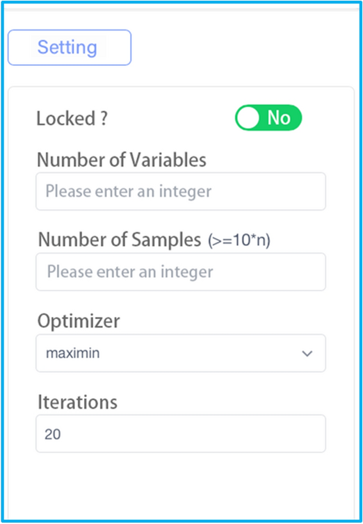
The parameter configuration pane of the LHS block
After the parameter is configured, users need to deploy and run the block to generate samples by clicking the deploy and run button sequentially. Clicking the deploy button means that what the users have done in the front-end (i.e., in the main workspace), such as, dragging and dropping blocks, and tuning the parameters, will be updated to the back-end. When users ensure that all the operations and settings are correct, they can click the run button to run the workflow. During the running process, when a block is implemented successfully, the question mark icon in the block will turn to a green tick, as shown in Figure 8. This helps users keep track of the running state of the workflow.
Figure 8 
The identifier changes from the question mark to green tick when a block is implemented successfully
After the selected DoE block has been implemented successfully, users can visualize the spatial distribution of the generated samples by right-clicking the block and then clicking the plot button in the popped dialog. DoE blocks provide scatter plots, including 2D and 3D scatter plots, to help users visualize the samples. For the problems whose dimensionality is larger than three, users can select any two or three of the design variables to visualize the distribution of samples in the design space. In addition, users can set display options for the scatter plots, such as the color and size of the scatter points, axis limits, axis names, title, and font size. The sample data and scatter plot are all available for download.
-
(2)
Output evaluation module
Users can conduct simulations or experiments, using the downloaded sample data of design variables, to obtain the output evaluation. Then the samples of inputs and their corresponding outputs constitute the training samples for building a surrogate. There are two ways to fill in the output values in the parameter configuration pane of the output evaluation block: uploading an Excel file or filling out the form manually. Considering that there may exist invalid output evaluations, for instance, the simulation may not converge under particular parameter combinations, and some experimental results may be found incorrect, DADOS allows users to disable or enable any samples or design variables by clicking the boxes next to them. As shown in Figure 9, the 11th sample is disabled by clicking the box near the number 11. In addition, to make it easy for users to check the data, the background color of each row is designed as an alternative and when users hover over a sample data, the corresponding row and column will be highlighted.
Figure 9 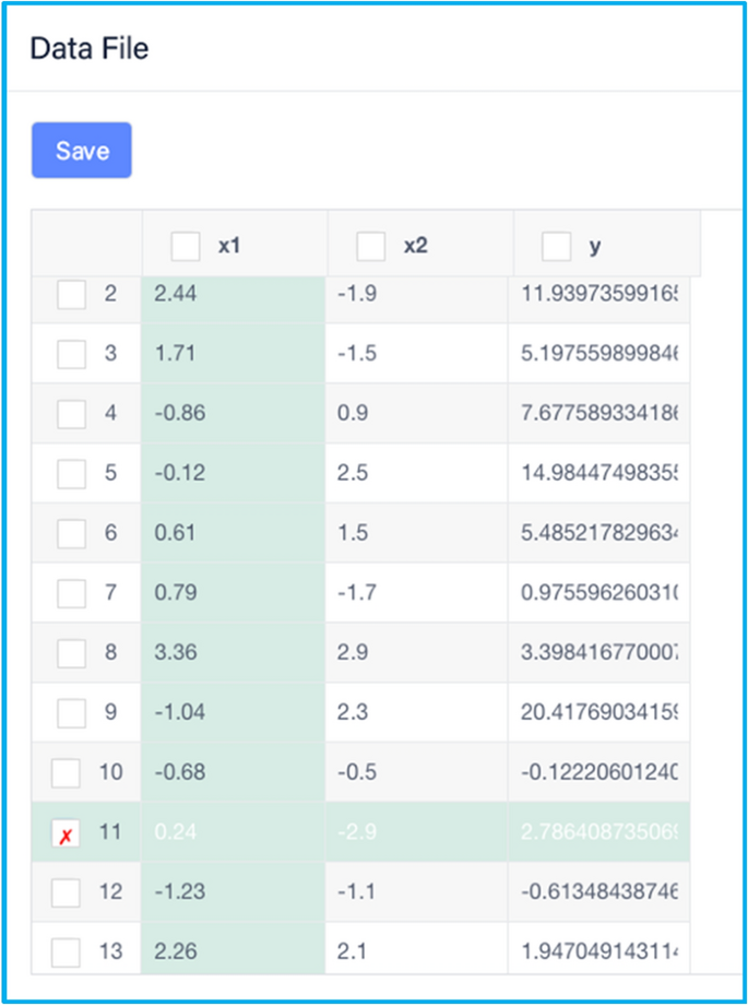
The data entry form of the output evaluation block
-
(3)
Surrogate model module
Surrogate model module includes six individual surrogate techniques (i.e., PRS, MLS, RBF, KRG, SVR, and ANN) and a unique ensemble surrogate technique (i.e., E-AHF) proposed by ourselves. To make it easier for users to configure the surrogate blocks, DADOS provides default parameter values. In addition, the details of parameter configuration can refer to the documentation page of DADOS. The E-AHF block allows users to select any combination of the individual surrogate techniques, as shown in Figure 10.
Figure 10 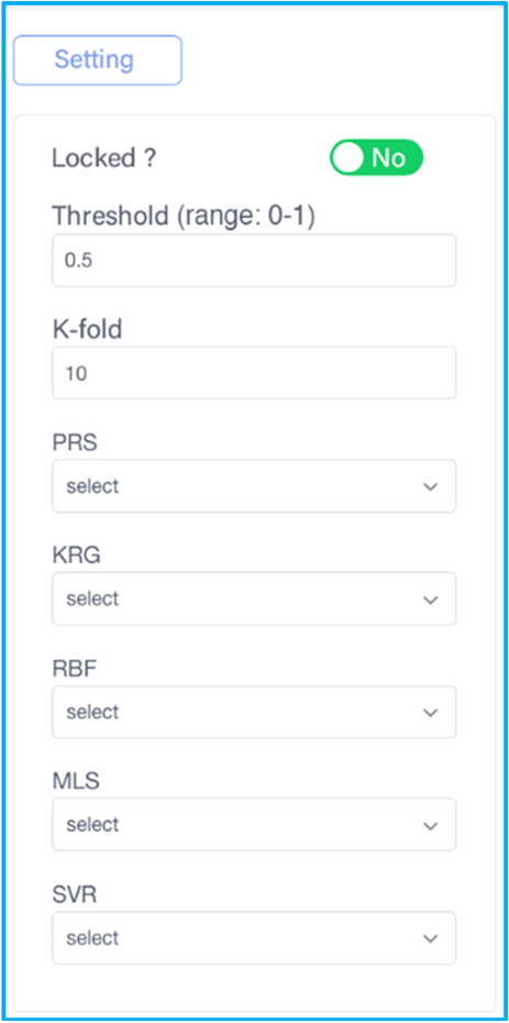
The configuration pane of the E-AHF block
After the surrogate model has been built successfully, users can visualize the response surface of the surrogate to gain insights into the relationship between inputs and outputs of the problem. DADOS provides 2D, 3D, and contour plots for the surrogate blocks. For the 3D plot, users can rotate and zoom it for a better view. In addition, DADOS supports data cursor mode, which allows users to select an individual data point to display its information. All the plots allow users to set display options and are available for download.
-
(4)
Model selection and validation module
DADOS employs LOOCV and k-fold CV to help users validate and select surrogate models due to the fact that CV allows the use of most of the available samples, even all the samples but one, to construct the surrogates, which saves computational burden and/or experimental cost to some extent compared to the split sample method. For the k-fold CV block, users need to specify the value of k in the parameter configuration pane. It is recommended that k should be a divisor of the number of total samples. That is, each fold has the exact same number of samples. In some cases, even if the number of total samples is not divisible by k, the algorithm will make the number of samples of each fold as even as possible. In DADOS, there are three available metrics, i.e., RMSE, \({R}^{2}\), and MAE, to validate the performance of surrogates.
-
(5)
Infill module
Infill module includes three infilling strategies that are mean squared error based exploration, PoI, and EI. Apart from choosing the infilling strategies, users are also allowed to choose the number of infilling samples in each infilling.
-
(6)
Y_infill module
Y_infill is a block that follows infill block to enable users to fill in the outputs of the infilling samples. The parameter configuration pane of Y_infill is very similar to that of Y_DOE block, which also supports users to upload an Excel file or fill out the form manually. Since there are just a few, even a single infilling sample during each infilling process, filling out the form manually would be a better choice. After the Y_infill block is configured, that is, samples have been updated, the surrogate can be trained again, using the updated samples, by dragging a new surrogate block into the canvas and connecting it to the Y_infill.
-
(7)
Pred module
Pred is a block that provides a fast prediction of the performance of a new design. Similar to Y_DOE and Y_infill block, users can fill in new combinations of design variables to get fast predictions by uploading an Excel file or filling out the form manually.
-
(8)
Optimization module
The optimization blocks are linked right behind the surrogate or CV blocks to provide an optimal design based on the established surrogate model. Since an optimization problem can be generally formulated by an objective function and several constraint functions, DADOS has a built-in formula editor for users to edit equations. In the parameter configuration pane of the optimization blocks, as shown in Figure 11, users can not only tune the parameters of the optimization algorithm but also can specify the number of constraint functions and formulate the objective and constraint functions using the established surrogates. In addition, the iteration step plot is available in the optimization blocks.
Figure 11 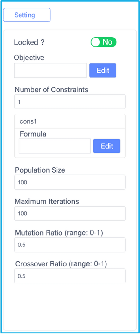
The parameter configuration pane of the GA block
-
(9)
Sensitivity analysis module
Like the prediction and optimization blocks, the sensitivity analysis blocks are also linked right behind the surrogate or CV blocks. They can provide an evaluation of how much each input variable is contributing to the output uncertainty. There are four available SA methods in DADOS, i.e., FAST, Sobol, Morris, and DELTA, among which, FAST and Sobol blocks provide a bar plot to show first order index and total order index.


4 Examples
In this section, a numerical example and a real-world engineering problem are used to demonstrate how to use DADOS to conduct data-driven design optimization.
4.1 Numerical Example
The numerical example is an unconstrained global optimization test function adopted from Ref. [47], named McCormick function. The formula of McCormick function is expressed as follows:
where, \({x}_{1}\) and \({x}_{2}\) are two design variables and the domain is \({x}_{1}\in \left[-1.5, 4\right], {x}_{2}\in [-3, 4]\). This function has one global minimum \(f\left({{\varvec{x}}}^{\boldsymbol{*}}\right)\approx -1.913\) at \({{\varvec{x}}}^{\boldsymbol{*}}=(-0.547,-1.547)\).
Let us assume that the McCormick function is expensive to evaluate and its formula is unknown. Only the range of the design space and some samples drawn from it are available. In the following, what will be done is using the available samples to build a surrogate to approximate the true function in Eq. (9), trying to find its global minimum, and analyzing which variable has more impact on the output.
First of all, users need to create a project by clicking the new button as shown in Figure 4. Then, basic information about the project should be entered. After the project is created, users need to open the project to start the task. When users open the project, the main workspace becomes available as shown in Figure 12. Then, step-by-step instruction for using DADOS to find the optimal value of the unknown function in Eq. (9) is detailed as follows:
-
Step 1: Start. Drag the start block from the left pane Algorithm blocks and drop it on the canvas. The start block indicates the beginning of the project and there is only one start block in a project.
-
Step 2: DoE. In this step, the OLHS sampling plan is chosen to generate the samples. Drag the OLHS block from the DoE module and drop it on the canvas. In the parameter configuration pane of the block, four parameters need to be configured and two of them are set by default. Hence, users just need to configure the other two parameters, that is, number of variables and number of samples. When users enter 2 in the box under number of variables, sub-boxes containing the interval, precision, and name of variable are shown up just under number of variables box, as shown in Figure 13. Users need to fill these boxes accordingly. Then, users link the OLHS block to the start block and click the deploy and run button sequentially to generate the samples of inputs. Next, click the corresponding name of the OLHS block in the results pane to view and download the data of samples of inputs.
-
Step 3: Output evaluations. In this step, users need to upload the samples of inputs and the corresponding output values to DADOS via Y_DOE block. Specifically, calculate the output values to samples of inputs using Eq. (9) and fill them in the Excel file that is downloaded from Step 2. Then, drag the Y_DOE block from the left pane, drop it on the canvas, and link the Y_DOE block to the OLHS block. In the configuration pane, as shown in Figure 14, click the cloud icon to upload the Excel file and fill in the name of responses in the Remarks box.
-
Step 4: Construction of surrogate models. In this step, a surrogate model is constructed using the E-AHF method. Drag the E-AHF block from the left pane, drop it on the canvas, and link the E-AHF block to the Y_DOE block. As shown in Figure 15, in the configuration pane, five individual surrogates are selected by default to form the ensemble surrogate. Click the deploy and run button sequentially to run the workflow. Note that when the question mark of each block turns to a green tick, it denotes that the workflow has been run successfully. There is something wrong if not all the blocks have a green tick and users can read the running log to debug the workflow.
-
Step 5: Model validation. This step checks the accuracy of the surrogate model built in the previous step. Drag the LOOCV block and drop it on the canvas. There are three metrics available to choose in the configuration pane: \({R}^{2}\), RMSE and MAE. All three metrics are chosen by default. Then, link the LOOCV block to the E-AHF block and, click the deploy and run button. But before deploying and running the workflow, it would be better to turn the lock button on in the configuration pane of the E-AHF block. The lock button of a block being on indicates that all the previous blocks and this block are locked and will not run again to waste computational resources. Because all the information related to the modeling process will transfer to the next block by the link, there is no need to run the previous blocks again and only the current block is required to be implemented. After the LOOCV block was implemented, users can check the accuracy of the E-AHF model in results pane, and the results are listed in Table 1. As mentioned in Refs. [48] and [9], \({R}^{2}\)> 0.8 indicates a surrogate with good predictive accuracy. The surrogate model is more accurate if \({R}^{2}\) is closer to 1. Therefore, we set \({R}^{2}\)> 0.8 as a threshold to determine that a surrogate model is satisfied. For RMSE and MAE, it is difficult or even impossible to find the threshold to judge whether a surrogate model is satisfied, because the values of the RMSE and MAE depend on the problems. For different problems, the range of RMSE and MAE varies with the responses. However, with RMSE and MAE, we can determine which surrogate is better than others.
-
Step 6: Optimization. In this step, a Genetic Algorithm (GA) was employed to optimize the E-AHF model. Drag the GA block from the left pane, drop it on the canvas, and link it to the LOOCV block. As shown in Figure 16, in the configuration pane, users need to specify the objective and constraints. To edit the objective function, users need to click the edit button next to the objective box to open the formula editor. In the popped formula editor, users can choose to conduct minimization or maximization by clicking the drop-down menu, as shown in Figure 17. Moreover, users can edit the objective function using the variable names listed in the editor. For this numerical example, minimization is selected and the objective function is y1, which denotes minimizing the response of the E-AHF model. The other parameters of GA are set to default. Next, click the deploy and run button sequentially to run the workflow. After the GA block was implemented, users can see the optimization results in results pane and view the iteration step plot by right clicking the GA block and clicking the plot button in the popped dialog. The optimization results and the iteration step plot are shown in Table 2 and Figure 18, from which it can be observed that the optimized results are in very good agreement with the global minimum.
-
Step 7: Sensitivity analysis. In this step, a Sobol method was employed to conduct sensitivity analysis. Drag the SOBOL block from the left pane, drop it on the canvas, and link it to the LOOCV block. In the parameter configuration pane, as shown in Figure 19, setting the number of samples to 10000. Next, click the deploy and run button sequentially to run the workflow. The first-order index and total order index are shown in Figure 20, denoted by S1 and ST, respectively. It can be observed from Figure 20 that the interaction between \({x}_{1}\) and \({x}_{2}\) has a great impact on the output of the McCormick function.

The blank main workspace screen of DADOS

Configuration of the OLHS block for the numerical example

Configuration of the Y_DOE block for the numerical example

Configuration of the E-AHF block for the numerical example

Configuration of the GA block for the numerical example

The formula editor in DADOS

The iteration plot of the GA block

Configuration of the Sobol block for the numerical example

The first-order index and total order index
4.2 Engineering Case
In this section, we use DADOS to conduct structural optimization in lightweight design for a mining hoist sheave. In underground mining, a hoist is used to raise and lower conveyances within the mine shaft. The sheave is an important part of the hoist system, which is a wheel with an open groove that a cable fits around so it can rotate around the exterior. One end of the cable is attached to conveyances, while the other is attached to a fixed object. The high demand for mining hoists, such as high speed, heavy load, and stability, drives the sheave to be cumbersome, which makes it more challenging to transport, install, and maintain the sheave. Hence, the lightweight design of the sheave is of great importance. To make the sheave lighter, two types of eight lightening holes are designed in the sheave, as shown in Figures 21 and 22, \({x}_{1}\) to \({x}_{8}\) are eight structural parameters of lightening holes. These structural parameters are optimized to minimize the weight of the sheave under the maximum stress constraints. Figure 22 shows the stress distribution and location of the maximum stress when the sheave is subjected to the maximum radial force at \({45}^{^\circ }\). This optimization problem can be formulated as Eq. (10):
where \(f\left(x\right)\) is the weight of the designed hoist sheave, \({g}_{1}\left(x\right)\) and \({g}_{2}\left(x\right)\) are the maximum stresses when the sheave is subjected to the maximum radial force at \({0}^{^\circ }\) and \({45}^{^\circ }\), respectively.

Structural parameters of lightening holes in a mining hoist sheave

Stress distribution and the location of maximum stress under a maximum radial force at \({45}^{^\circ }\)
A step-by-step instruction of using DADOS to conduct this structural optimization problem is presented as follows:
-
Step 1: Start. Drag the start block from the left pane Algorithm blocks and drop it on the canvas.
-
Step 2: DoE. In this step, the OLHS sampling plan is chosen to generate the samples. Drag the OLHS block from the DoE component, drop it on the canvas, and link it to the start block. In the parameter configuration pane of the OLHS block, set the number of design variables and samples to 8 and 175, respectively. The domain of the 8 design variables is set according to Eq. (10). Then, click the deploy and run button sequentially to generate the samples of inputs.
-
Step 3: Output evaluations. In this step, users need to upload the samples of inputs and the corresponding output values to DADOS via Y_DOE block. Conducting simulations according to the samples of inputs generated in the previous step to obtain the corresponding mass and maximum stress when the maximum radial force is applied at \({0}^{^\circ }\) and \({45}^{^\circ }\), respectively. Drag the Y_DOE block from the left pane, drop it on the canvas, and link it to the OLHS block. Repeat this process three times to have three Y_DOE blocks on the canvas. Upload the data of mass, maximum stress to these three Y_DOE blocks, respectively. Then, click the deploy and run button sequentially to run the workflow.
-
Step 4: Construction of surrogate models. In this step, one E-AHF and two RBF models are constructed to approximate the relationship between the design variables and the mass, maximum stress when the maximum radial force at \({0}^{^\circ }\) and \({45}^{^\circ }\), respectively. Drag an RBF block, an E-AHF block, and another RBF block from left pane, drop them on the canvas, and link them to the three Y_DOE blocks respectively. For parameter configurations, the multiquadratic function was chosen as the basis function for the two RBF models, and the parameters of the E-AHF model are set to default. Then, click the deploy and run button sequentially to run the workflow.
-
Step 5: Model validation. In this step, the 10-fold CV was employed to evaluate the accuracy of the three surrogate models and the results are shown in Table 3.
-
Step 6: Optimization. In this step, a GA method was employed to optimize the weight of the hoisting sheave with stress as constraints. Drag a GA block from the left pane, drop it on the canvas, and link the three surrogate blocks to it. In the parameter configuration pane of the GA block, click the edit button next to the objective box, then type y1, which represents the mass of the sheave, in the popped formula editor and choose min from the drop-down menu. Next, specify two inequality constraints and type y2-51 and y3-51 in the formula editor. Then, click the deploy and run button sequentially to run the workflow. By running the simulation according to the optimized structural parameters, the weight and maximum stresses of the optimized sheave are obtained and listed in Table 4. Compared to the initial sheave weight of 4844.78 kg, the optimized weight is 4599.60 kg, which is a reduction of 5.06%.
5 Conclusions
This paper introduces a cloud-based data-driven design optimization system, DADOS, to help engineers, researchers and especially beginners improve a design or product easily and efficiently. The architecture and interface of DADOS were detailed in the paper. A numerical function and a practical problem were used to demonstrate how to use DADOS to conduct data-driven design optimization in a step-by-step way. DADOS has the following features.
-
(1)
The current version of DADOS has nearly 30 key algorithms, including design of experiments, surrogate models, model validation and selection, prediction, optimization, and sensitivity analysis, which are fundamental for users to conduct design optimization. DADOS has an exclusive robust hybrid surrogate technique that seeks to make use of advantages of each individual surrogate and to eliminate the effort of selecting the appropriate individual.
-
(2)
DADOS employed flow-based programming so that users can conduct design optimization easily just by assembling drag-and-drop algorithm blocks and without the need to write any code.
-
(3)
Since DADOS is cloud-based software, there is no need to download and install it, users can apply it via a web browser at any time, any place, and for free, as long as they can be linked to the internet.
-
(4)
DADOS allows multi-person working on a project at the same time and supports multi-disciplinary optimization.
Apart from the above-mentioned features, DADOS is now in its first version. There is still a long way for it to go. We will continuously maintain and develop DADOS in the future. On the one hand, aesthetics of the user interface and usability of DADOS will be improved further. On the other hand, more algorithm blocks will be added to expand the existing modules in DADOS, and new modules will be developed to provide more functions for users, such as multi-fidelity surrogate models, uncertainty quantification, reliability-based optimization, etc. We hope DADOS can be an effective tool to help engineers and researchers conduct design optimization, and we sincerely welcome peers to join us to shape DADOS for better functionality and usability.
Data availability
The data that support the findings of this study are available on request from the authors.
References
J Martins, A B Lambe. Multidisciplinary design optimization: A survey of architectures. AIAA Journal, 2013, 51(9): 2049–2075.
A Bertoni. Data-driven design in concept development: Systematic review and missed opportunities. Proceedings of the Design Society: DESIGN Conference, 2020, 1: 101–110.
F A C Viana, T W Simpson, V Balabanov, et al. Metamodeling in multidisciplinary design optimization: How far have we really come? AIAA Journal, 2014, 52(4): 670–690.
H Wang, F Ye, L Chen, et al. Sheet metal forming optimization by using surrogate modeling techniques. Chinese Journal of Mechanical Engineering, 2017, 30(1): 22–36.
S Deshpande, L T Watson, J Shu, et al. Data driven surrogate-based optimization in the problem solving environment WBCSim. Engineering with Computers, 2011, 27(3): 211–223.
S N Lophaven, H B Nielsen, J Sondergaard. DACE - A Matlab Kriging Toolbox. Kgs. Lyngby, Denmark, version 2.0, 2002[2022-11-20], https://www.omicron.dk/dace/dace.pdf.
I Couckuyt, T Dhaene, P Demeester. OoDACE toolbox: A flexible object-oriented kriging implementation. Journal of Machine Learning Research, 2014, 15: 3183–3186.
I Couckuyt, A Forrester, D Gorissen, et al. Blind Kriging: Implementation and performance analysis. Advances in Engineering Software, 2012, 49(1): 1–13.
A Forrester, A Sóbester, A J Keane. Engineering design via surrogate modelling: a practical guide. New York: John Wiley & Sons, Inc., 2008.
FAC Viana, SURROGATES Toolbox User's Guide. Gainesville, FL, USA, version 3.0, 2011[2022-11-20], https://sites.google.com/site/srgtstoolbox.
D Gorissen, I Couckuyt, P Demeester, et al. A surrogate modeling and adaptive sampling toolbox for computer based design. Journal of Machine Learning Research, 2010, 11: 2051–2055.
M Juliane. MATSuMoTo code documentation. Ithaca, NY, USA, 2014[2022-11-20], https://github.com/Piiloblondie/MATSuMoTo.
M A Bouhlel, J T Hwang, N Bartoli, et al. A Python surrogate modeling framework with derivatives. Advances in Engineering Software, 2019, 135: 102662.
Y Liu, T Zhang, Y Gao, et al. A MATLAB GUI toolbox for surrogate-based design and optimization. 9th IEEE International Conference on Cyber Technology in Automation, Control and Intelligent Systems, CYBER 2019, IEEE, 2019: 103–106.
A K Das, S Dewanjee. Optimization of extraction using mathematical models and computation. Computational Phytochemistry. 2018, 75–106.
S S Garud, I A Karimi, M Kraft. Design of computer experiments: A review. Computers & Chemical Engineering, 2017, 106: 71–95.
J A Palasota, S N Deming. Central composite experimental designs. Journal of Chemical Education, 1992, 69(7): 560–563.
M Chien, T Hyungmin. Stochastic bending and buckling analysis of laminated composite plates using Latin hypercube sampling. Engineering with Computers, 2021: 1–39.
N V Queipo, R T Haftka, W Shyy, at al. Surrogate-based analysis and optimization. Progress in Aerospace Sciences, 2005, 1(41): 1–28.
X He, L Yang, R Ran, et al. Comparative studies of surrogate models based on multiple evaluation criteria. Journal of Mechanical Engineering, 2022, 58(16): 403–419. (in Chinese)
K Li, S Wang, Y Liu, et al. An integrated surrogate modeling method for fusing noisy and noise-free data. Journal of Mechanical Design, 2022, 144(6): 061701.
Z Majdisova, V Skala. Radial basis function approximations: comparison and applications. Applied Mathematical Modelling, 2017, 51: 728–743.
Y Liu, S Wang, Q Zhou, et al. Modified multifidelity surrogate model based on radial basis function with adaptive scale factor. Chinese Journal of Mechanical Engineering, 2022, 35: 77.
C E Rasmussen, H Nickisch. Gaussian processes for machine learning (GPML) toolbox. Journal of Machine Learning Research, 2010, 11: 3011–3015.
Z Zhai, H Li, X Wang. An adaptive sampling method for Kriging surrogate model with multiple outputs. Engineering with Computers, 2020: 1-19.
H Xiang, Y Li, H Liao, et al. An adaptive surrogate model based on support vector regression and its application to the optimization of railway wind barriers. Structural and Multidisciplinary Optimization, 2017, 55(2): 701–713.
K Parand, M Razzaghi, R Sahleh, et al. Least squares support vector regression for solving Volterra integral equations. Engineering with Computers, 2020: 1-8.
M Mohammadhassani, H Nezamabadi-Pour, M Z Jumaat, et al. Artificial neural networks: fundamentals, computing, design, and application. Journal of Microbiological Methods, 2000, 43(1): 3–31.
L Zhang, T Li, J Zhang, et al. Optimization on the crosswind stability of trains using neural network surrogate model. Chinese Journal of Mechanical Engineering, 2021, 34: 86.
S Wang, X Lai, X He, et al. Building a trustworthy product-level shape-performance integrated digital twin with multifidelity surrogate model. Journal of Mechanical Design, 2022, 144(3): 031703.
S Wang, Y Liu, Q Zhou, et al. A multi-fidelity surrogate model based on moving least squares: fusing different fidelity data for engineering design. Structural and Multidisciplinary Optimization, 2021, 64(6): 3637–3652.
L Lv, C Zong, C Zhang, et al. Multi-fidelity surrogate model based on canonical correlation analysis and least squares. Journal of Mechanical Design, 2021, 143(2): 1–17.
F A C Viana, R T Haftka, Surrogate-based optimization with parallel simulations using the probability of improvement. 13th AIAA/ISSMO Multidisciplinary Analysis Optimization Conference, Texas, USA, September 13-15, 2010: 9392.
Y Zhang, S Wang, C Zhou, et al. A fast active learning method in design of experiments: multipeak parallel adaptive infilling strategy based on expected improvement. Structural and Multidisciplinary Optimization, 2021, 64(3): 1259–1284.
D. Whitley. A genetic algorithm tutorial. Statistics and Computing, 1994, 4(2): 65–85.
M O Okwu, L K Tartibu. Particle swarm optimisation. Studies in Computational Intelligence, 2021, 927: 5–13.
S Kirkpatrick, C D Gelatt, M P Vecchi, Optimization by simulated annealing. Science, 1983, 220(4598): 671–680.
A A Heidari, S Mirjalili, H Faris, et al. Harris hawks optimization: Algorithm and applications. Future Generation Computer Systems, 2019, 97: 849–872.
M M J Opgenoord, D L Allaire, K E Willcox. Variance-based sensitivity analysis to support simulation-based design under uncertainty. Journal of Mechanical Design, 2016, 138(11): 111410.
I M Sobol, S Kucherenko. Derivative based global sensitivity measures. Procedia-Social and Behavioral Sciences, 2010, 2(6): 7745–7746.
I M Sobol. Global sensitivity indices for nonlinear mathematical models and their Monte Carlo estimates. Mathematics and Computers in Simulation, 2001, 55(1–3): 271–280.
A Saltelli, R Bolado. An alternative way to compute Fourier amplitude sensitivity test (FAST). Computational Statistics and Data Analysis, 1998, 26(4): 445–460.
M D Morris. Factorial sampling plans for preliminary computational experiments. Technometrics, 1991, 33(2): 161–174.
E Borgonovo. A new uncertainty importance measure. Reliability Engineering and System Safety, 2007, 92(6): 771–784.
X Song, L Lv, J Li, et al. An advanced and robust ensemble surrogate model : Extended adaptive hybrid functions. Journal of Mechanical Design, 2018, 140(2): 1–9.
X J Zhou, T Jiang. Metamodel selection based on stepwise regression. Structural and Multidisciplinary Optimization, 2016, 54(3): 641–657.
J Tao, G Sun. Application of deep learning based multi-fidelity surrogate model to robust aerodynamic design optimization. Aerospace Science and Technology, 2019, 92: 722–737.
L Lv, M Shi, X Song, et al. A fast-converging ensemble infilling approach balancing global exploration and local exploitation: The Go-inspired hybrid infilling strategy. Journal of Mechanical Design, 2020, 142(2): 021403.
Acknowledgements
The authors would like to thank Liye Lv, Lin Zhang, Yanan Zou, Peng Cui, and Yang Zhang for their efforts in developing DADOS.
Funding
Supported by National Key Research and Development Program of China (Grant No. 2018YFB1700704) and National Natural Science Foundation of China (Grant No. 52075068).
Author information
Authors and Affiliations
Contributions
XS and SW were in charge of the development of the software and the whole trial; SW wrote the manuscript; YZ assisted with the development of the software and the whole trial; YL and KL revised the manuscript and assisted with the whole trial. All authors read and approved the final manuscript.
Authors’ Information
Xueguan Song born in 1982, is currently a professor at School of Mechanical Engineering, Dalian University of Technology, China. His research interests include multidisciplinary design optimization, surrogate modeling, mechanical design, digital twin, and computational fluid dynamics.
Shuo Wang born in 1993, is currently a PhD candidate at School of Mechanical Engineering, Dalian University of Technology, China. His research interests include multidisciplinary design optimization, surrogate modeling, and digital twin.
Yonggang Zhao born in 1994, is currently an assistant engineer at AECC Shenyang Engine Research Institute, China. He received his master degree from School of Mechanical Engineering, Dalian University of Technology, China in 2021.
Yin Liu born in 1992, is currently a PhD candidate at School of Mechanical Engineering, Dalian University of Technology, China. Her research interests include surrogate modeling and sequential sampling strategy.
Kunpeng Li born in 1992, is currently a PhD candidate at School of Mechanical Engineering, Dalian University of Technology, China. His research interests include multidisciplinary design optimization, surrogate modeling, and digital twin.
Corresponding authors
Ethics declarations
Competing interests
The authors declare no competing financial interests.
Rights and permissions
Open Access This article is licensed under a Creative Commons Attribution 4.0 International License, which permits use, sharing, adaptation, distribution and reproduction in any medium or format, as long as you give appropriate credit to the original author(s) and the source, provide a link to the Creative Commons licence, and indicate if changes were made. The images or other third party material in this article are included in the article's Creative Commons licence, unless indicated otherwise in a credit line to the material. If material is not included in the article's Creative Commons licence and your intended use is not permitted by statutory regulation or exceeds the permitted use, you will need to obtain permission directly from the copyright holder. To view a copy of this licence, visit http://creativecommons.org/licenses/by/4.0/.
About this article

Cite this article
Song, X., Wang, S., Zhao, Y. et al. DADOS: A Cloud-based Data-driven Design Optimization System. Chin. J. Mech. Eng. 36, 34 (2023). https://doi.org/10.1186/s10033-023-00857-x
Received:
Revised:
Accepted:
Published:
DOI: https://doi.org/10.1186/s10033-023-00857-x