- Original Article
- Open access
- Published:
Similar Vertices and Isomorphism Detection for Planar Kinematic Chains Based on Ameliorated Multi-Order Adjacent Vertex Assignment Sequence
Chinese Journal of Mechanical Engineering volume 34, Article number: 20 (2021)
Abstract
Isomorphism detection is fundamental to the synthesis and innovative design of kinematic chains (KCs). The detection can be performed accurately by using the similarity of KCs. However, there are very few works on isomorphism detection based on the properties of similar vertices. In this paper, an ameliorated multi-order adjacent vertex assignment sequence (AMAVS) method is proposed to seek out similar vertices and identify the isomorphism of the planar KCs. First, the specific definition of AMAVS is described. Through the calculation of the AMAVS, the adjacent vertex value sequence reflecting the uniqueness of the topology features is established. Based on the value sequence, all possible similar vertices, corresponding relations, and isomorphism discrimination can be realized. By checking the topological graph of KCs with a different number of links, the effectiveness and efficiency of the proposed method are verified. Finally, the method is employed to implement the similar vertices and isomorphism detection of all the 9-link 2-DOF(degree of freedom) planar KCs.
1 Introduction
The multi-component and multi-DOF mechanism is widely used in various mechanical equipment, involving engineering machinery, medical machinery, agricultural machinery. The innovative design of mechanism structure is still the critical step of product upgrading [1]. The correct solution of the similar vertices [2] can not only reduce the number of isomorphism detection but also provide a theoretical basis for the selection of rack, input, and output components. In 1992, Yan [3] proposed a new mechanism design technology, called regenerative KCs method, which essentially represents the logical reasoning of the regeneration process of KCs. In logic reasoning, the similar vertices should be analyzed to improve the efficiency of innovative design and reduce redundant design scheme. In the same year, Hwang [4] divided the similarity into symmetry similarity, transfer similarity, row similarity, and irregular similarity, and proposed the relationship code method of the weighted line graph to distinguish the similar vertices of functional components. Although Hwang’s method is simple, it has a situation of misjudgment.
In mechanism synthesis, isomorphism detection is fundamental. Many works have been done, and a large number of methods and theories have been developed. Kong et al. [5] first applied the artificial neural network technology for isomorphism detection and established the neural network model of topological graphs. Chang et al. [6] proposed an eigenvalue and eigenvector-based method to identify KCs isomorphism for the first time. Cubillo and Wan [7] proposed the necessary and sufficient conditions for eigenvalues and eigenvectors of isomorphic KCs; Later, Sunkari and Schmidt [8] found that this method has certain limitations, i.e., counterexamples will appear when the number of components in the KCs is greater than 14. Xiao et al. [9] creatively combined ant colony algorithms and artificial immune algorithms to identify the isomorphism of KCs. Galán-Marín et al. [10] first used the multi-value neural network method to identify the isomorphism of KCs. In the same year, Dargar et al. [11] identified isomorphism by comparing the first-order and second-order adjacent component values of the KCs, but it cannot describe the uniqueness of each vertex in the topological graph. Yang et al. [12] proposed a method to detect isomorphism based on the correlation matrix of KCs. By using this method, the sufficiency of isomorphism detection was obtained based on vertex correspondence. Other isomorphism detection methods, such as partition matching algorithm [13], hybrid immune algorithm [14], optimized circuit simulation [15,16,17], connectivity number and entropy [18], binary code [19], information theory [20], joint matrix [21, 22], loop theory [23,24,25,26], high-order adjacency link values [27], are noticeable too.
Although all the abovementioned synthesis methods can identify the isomorphism, they cannot accurately find the similar vertices that are beneficial for mechanism selection and isomorphism detection. Hence, in this paper, an ameliorated multi-order adjacent vertex assignment sequence is proposed. The new method attempts to achieve similar vertices detecting and to ease the identification of isomorphism.
The rest of the paper is organized as follows: Section 2 describes the basic concepts of graph theory. In Section 3, the initial value rule and the definition of AMAVS of topological graphs are presented, and several examples are delivered to illustrate the detection of similar vertices. In Section 4, based on the correct solution of the similar vertices, the concrete steps of isomorphism detection of the KCs are given. Section 5 concludes this work.
2 Basic Concepts
2.1 Topological Model of KCs
KCs can be described by an undirected topological graph in which the vertices and edges represent the components and joints, respectively; The link relationship between vertices can be expressed by an adjacency matrix \(\varvec{A} = [a_{ij} ]_{n \times n}\), where n is the total number of vertices in the topological graph, and the adjacency matrix is a real symmetric matrix. The value rules of each element are as follows:
The degree of vertex i in a topological graph is defined as the number of edges connected with vertex i; it can also be determined by the sum of the ith column (row) of the adjacency matrix A. As shown in Figure 1, the topological graph of the 9-link 2-DOF KC is expressed as (b), and the corresponding adjacency matrix is A. Vertices 2, 4, 6, 7, and 9 are two-degree vertices, while vertices 1, 3, 5 and 8 are three-degree vertices.

2-DOF KCs (a) and its corresponding topological graph (b)
2.2 Definition of Similar Vertices
We consider a graph as a labeled graph when its vertices are labeled by the integers 1, 2, …, n. Due to different labeling, the vertices in the labeled graph have some interference characteristics. Thus, a characteristic constant not affected by the label is adopted to describe vertices for finding similar vertices. Additionally, in a topological graph, similar vertices have geometric symmetry so that two similar vertices must be symmetrical about a vertex or an edge, which means that the similar vertices must have the same characteristic constant. In this paper, an AMAVS is employed as a criterion for similarity detection. The vertices with the same AMAVS are similar and vice versa.
2.3 Isomorphism of KCs
If one-to-one mapping f exists for the two graphs \(G_{1} = (V_{1} ,E_{1} )\) and \(G_{2} = (V_{2} ,E_{2} )\), and the following expression is satisfied:
Then graphs G1 and G2 are isomorphic. As shown in Figure 2, G(a) and G(b) are isomorphic.

Isomorphic topological graph
2.4 Degree of a Vertex
The degree of a vertex is defined as the number of edges incident with that vertex. For the graph G(a) shown in Figure 2, the degree of vertex 2, 4, 7, and 9 is three, whereas vertex 1, 3, 5, 6, and 8 is two [28].
3 AMAVS and Solution of Similar Vertices
3.1 Initial Value and AMAVS
For any given topological graph, the number of 3j of the Fibonacci sequence [29, 30] is assigned according to the size of each vertex degree, where j is a positive integer. According to the vertex degrees, the values of j are 1, 5, 21, 89, ….
Due to the characteristics of the Fibonacci sequence, the sum of two groups with the same number of Fibonacci numbers is usually different. For example, for the first four items 1, 5, 21, 89 of the selected Fibonacci sequence, the sum of two repeatable pairs is carried out, and the result is 2, 6, 10, 22, 26, 42, 90, 94, 110, 178; for the natural number 1, 2, 3, 4, the result is 2, 3, 4, 4, 5, 5, 6, 6, 7, 8. Compared with other sequences, the Fibonacci sequence can significantly reduce the repetition of high-order values, which better reflects the characteristics of vertices.
The vertices with equal degrees are assigned the same value, which is defined as the initial assignment. Moreover, the initial value sequence is recorded as \(S^{0}\). As shown in Figure 1(b), since vertices 2, 4, 6, 7, and 9 are two-degree vertices, the initial value of vertices 2, 4, 6, 7, and 9 is 1. Vertices 1, 3, 5, and 8 are three-degree vertices, so the initial value of vertices 1, 3, 5, and 8 is 5, i.e., the initial value sequence is \(S^{0}\) = {5, 1, 5, 1, 5, 1, 1, 5, 1}.
Note that the rth order adjacent vertex value (AVV) of vertex i in topological graph G is \(S_{i}^{r}\):
where n is the total number of vertices in a graph. \(a_{i,j}\) is the element corresponding to row i and column j of adjacency matrix A. \(S_{i}^{r - 1}\) is the (r−1)th order AVV of vertex i. It can be seen from the analysis that the larger r is, the more fully r-order AVV characterizes the vertex of the topological graph. Moreover, the larger r is, the more complex its calculation is. So it is of great significance to choosing the right r. In this paper, r is taken as the integral part of \(\sqrt n + d\), where d changes dynamically according to the specific situation.
The rules for changing the value of d are as follows:
-
Step 1: Let \(d = d_{0}\), \(r_{0}\) be the integer part of \(\sqrt n + d_{0}\), \(r_{1}\) be the integer part of \(\sqrt n + d_{0} + 1\), and \(d_{0}\) be the increasing integer value from 1.
-
Step 2: Using \(r_{0}\) and \(r_{1}\) to find similar vertices. If the results of the two groups of similar vertices are the same, set r as an integral part of \(\sqrt n + d_{0} + 1\), that is, the value of \(r_{1}\). If the results of two groups of similar vertices are different, \(d = d_{0} + 1\), and then repeat the above steps until the solving results of \(r_{0}\) and \(r_{1}\) are the same.
The comparing process can ensure the accuracy of the final results. The dynamic change of r verifies the final result to a certain extent, but it cannot guarantee the complete accuracy of the final result. There may be a mutation of the result after value r is determined. For example, when r is equal to 1, the result of similar vertices is the same as when r is 2, but when r is 3, the result is different. The determination of value r cannot achieve the complete accuracy of logic in theory, but no counterexample is found in the actual calculating process.
Herein, the value of the weighting part is set as 1/10 rather than 1/n. The significant advantage of this setting is that the decimal vertex of the AVV of order r is precisely equal to r, which can avoid rounding error.
The sequence of the r-order AVV of all vertices is \(S^{r} = \{ s_{1}^{r} ,s_{2}^{r} ,s_{3}^{r} , \ldots ,s_{n}^{r} \}\). The rth order AVV of vertex i is determined by the initial value of vertex i, the degree of vertex i, the degree of the vertex adjacent to vertex i and the (r−1)th order AVV of the vertex adjacent to vertex i. Hence, the rth order AVV can uniquely describe the characteristics of each vertex in the topological graph. That is, in the rth order AVV sequence \(S^{r}\), if the rth order AVV of two vertices is the same, these two vertices are similar; otherwise, they are not similar. The solution of similar vertices is of great significance to selecting the rack, input, and output components. The correct solution of similar vertices can reduce the number of isomorphism detection and improve the overall efficiency of mechanism synthesis.
3.2 Examples of Finding Similar Vertices
Example 1
As shown in Figure 3, the corresponding topological graph of the 11-link 2-DOF KCs (a) is shown in Figure 3(b). The process and results of finding similar vertices by using the AMAVS and the method in Ref. [23] are as follows.

a 11-link 2-DOF KCs and b its topological graph
The method in Ref. [23]: the value of r before correction is 4, the initial value of the prime number sequence according to the vertex degree of the topological graph is recorded as \(S^{0}\), and the fourth-order AVV sequence is recorded as S4, the solution results by the method in Ref. [23] are shown in Table 1.
According to the fourth-order AVV sequence S4, \(s_{6}^{4} = s_{9}^{4} = 2.7740\), vertices 6 and 9 are similar. However, there are no similar vertices in this topological graph. Considering whether the value of r is too small to obtain the correctness results, we also performed the similarity detecting of the fifth-, eighth-, and even eleventh-order AVV series. Not surprising results still illustrate that 6 and 9 are similar, which means that there are problems in the formula in Ref. [23].
Actually, in Ref. [23], the value of r is constant to 4, which leads to a relatively large amount of calculation for the KCs with a small number of components and could not guarantee the accuracy for the KCs with more components. The dynamic alteration of r in this paper can effectively ensure efficiency and accuracy. The formula for solving the high-order AVV is modified to eliminate the errors in Table 1. The new formula is more accurate to reflect the characteristic constants of each vertex, which can confirm whether the KCs are isomorphic when discriminating against similar vertices. The process of AMAVS is as follows.
The method of AMAVS: total vertices of topological graph n = 11, \(r_{0} = \sqrt n + 1 \approx 4\), \(r_{1} = \sqrt n + 2 \approx 5\). The initial value of the vertex degree in a topological graph is S0. By using the initial value, the fourth- and fifth-order AVV sequence obtained from Eq. (3) is recorded as S4 and S5. The specific solution results by the AMAVS method are shown in Table 2.
Since the adjacency values of each vertex in both fourth- and fifth-order AVV sequences S4 and S5 are entirely different, there are no similar vertices in the topological graph, which means that we can obtain eleven different mechanisms by choosing each vertex as a rack.
Example 2
Figure 4 shows a topological graph with 12 vertices and 15 edges. Hence, the order value r0 and r1 are equal to 4 and 5, respectively.

A topological graph with 12 vertices and 15 edges
The initial value of the vertex degree in the topological graph is S0; By using the initial value, the fourth and fifth-order AVV sequence obtained from Eq. (3) is recorded as S4 and S5. The specific solution results by the AMAVS method are shown in Table 3.
According to the fourth-order AVV sequence S4,
According to the fifth-order AVV sequence S5,
Upon these AVV sequences, the vertex in four vertex pairs, 1 and 6, 4 and 11, 5 and 10, 7 and 9, can be regarded as similar to each other, whereas other four vertices 2, 3, 8, and 12, with different adjacency values, are not similar. Therefore, we can obtain eight different mechanisms by choosing the corresponding vertex as a rack.
Example 3
Figure 5 shows a topology graph with 21 vertices and 29 edges. Hence, the order value r0 and r1 are equal to 5 and 6, respectively.

A topological graph with 21 vertices and 29 edges
The initial value of the vertex degree in the topological graph constructs a sequence, S0. The fifth- and sixth-order AVV sequences calculated from Eq. (3) are denoted as S5 and S6, respectively. The specific solution results by the AMAVS method are shown in Table 4.
According to the fifth-order AVV sequence S5,
According to the sixth order AVV sequence S6,
It is noteworthy that vertices in eight vertex pairs, 1 and 15, 2 and 16, 3 and 17, 4 and 6, 7 and 21, 8 and 19, 9 and 18, 14 and 20, are similar. Whereas the other five vertices 5, 10, 11, 12, and 13, with different adjacency values, are not similar. Therefore, for this KC, there are 13 different ways to choose the rack for mechanism innovation.
To further verifying the effectiveness, we also employ the proposed AMAVS method to detect the similar vertices of all the 9-link 2-DOF topological graphs, as shown in the Appendix. Meanwhile, the solution time given in Table 5 illustrates that the current study has a remarkable efficiency for detecting the similar vertices of the abovementioned graphs.
4 Steps and Examples of Isomorphic Detection
4.1 Initial Value and AMAVS
If the values of two sequences and the numbers of the same values are both the same, then the two sequences correspond to each other, and the corresponding relation is denoted as \({}_{a}^{b} M\). For example, two sequences Sa = {1, 3, 2, 4, 5} and Sb = 3, 4, 1, 5, 2}, can correspond to each other, and their corresponding relations from Sa to Sb is \({}_{a}^{b} M\) = {3, 1, 5, 2, 4}. The first element 3 of the corresponding relation indicates that the first element of the sequence Sa corresponds to the third element of the sequence Sb, the second element 1 of the corresponding relation indicates that the second element of the sequence Sa corresponds to the first element of the sequence Sb, and so on.
For any two isomorphic graphs, their corresponding vertex degrees must be the same, and the vertex degrees at the same distance from the two corresponding vertices must be the same [1]. As observed from Eq. (3), the rth order AVV of vertex i is determined by the initial value of vertex i, the degree of vertex i, the degree of the vertex adjacent to vertex i, and the (r−1)th order AVV of the vertex adjacent to vertex i. Thus, the corresponding relation \({}_{a}^{b} M\) can be established by the r-order AVV sequences \(S_{a}^{r}\) and \(S_{b}^{r}\). In order to identify the isomorphism graphs, a new adjacency matrix applied to compare with the reference graph G(b) can be obtained by interchanging the row and column of the initial adjacency matrix of topological graph G(a) following the corresponding relation \({}_{a}^{b} M\). If two adjacency matrices are the same, the two graphs are isomorphic, and vice versa. The isomorphism detection procedure is shown in Figure 6. The specific steps of isomorphism detection are described as follows.
-
Step 1: For any two given topological graphs G(a) and G(b), the initial values of each vertex degree are presented as \(S_{a}^{0}\) and \(S_{b}^{0}\). The r-order AVV sequences \(S_{a}^{r}\) and \(S_{b}^{r}\) are calculated by Eq. (3) to distinguish the similar vertices between G(a) and G(b). If the number of similar vertices of correspondence groups is different, the two topological graphs are non-isomorphic. Otherwise, go to step 2. If there are no similar vertices between the two topological graphs and the sequence \(S_{a}^{r}\) and \(S_{b}^{r}\) has no corresponding relation, the two graphs are non-isomorphic. Otherwise, there is a set of the corresponding relation \({}_{a}^{b} M\), and the program goes to step 5.
Figure 6 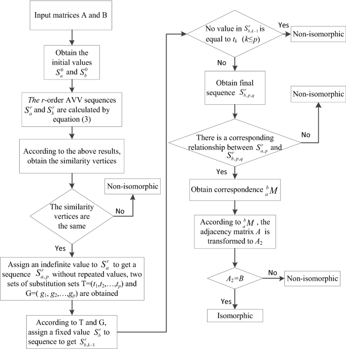
Isomorphism detection procedure
-
Step 2: The indefinite value of the sequence \(S_{a}^{r}\) is assigned according to the following rules: Select the vertex with the fewest similar vertices and the smallest label. Set the vertex label to i, change its initial value to the sum of the original initial value and the (p+1) Fibonacci number, where p is the number of indefinite assignment. For example, a vertex selected for the first initial value is j, its corresponding adjacent vertex value is recorded as t1, the new initial value of vertex j is recorded as g1, and its new r-order AVV sequence calculated by Eq. (3) is \(S_{a,1}^{r}\). If there are still duplicate values in \(S_{a,1}^{r}\), continue to assign indefinite values to the duplicate values until the sequence \(S_{a,p}^{r}\) without duplicate values. And two sets of substitution set T=(t1, t2,…, tp) and G=(g1, g2, …, gp) are obtained.
-
Step 3: The sequence \(S_{b}^{r}\) is assigned a fixed value according to T=(t1, t2,…, tp) and G=(g1, g2, …, gp). The specific rules are as follows: Obtain the same vertex as the first element t1 in the replacement set T of sequence \(S_{b}^{r}\), and assign a new initial value to this vertex as the first element g1 in the replacement set G, the new r-order AVV sequence \(S_{b,1}^{r}\) calculated by Eq. (3) according to the new initial value; Likewise, if the r-order AVV in the new sequence \(S_{b,1}^{r}\) is equal to t2, the new initial value given to the vertex is g2, and the new r-order AVV sequence calculated from Eq. (3) according to the new initial value is \(S_{b,2}^{r}\). If there are multiple values in \(S_{b,1}^{r}\) which are the same as t2, multiple new r-order AVV sequences \(S_{b,2}^{r}\) can be obtained. If no value in the sequence \(S_{b,k - 1}^{r}\) is equal to tk (k≤p) in the kth fixed value assignment process, the fixed value assignment fails, those two topological graphs are non-isomorphic, and the program terminates. Otherwise, one or more sets of final sequences \(S_{b,p,q}^{r}\) can be obtained, where q is the number of sets of final sequences.
-
Step 4: Compare the sequence \(S_{a,p}^{r}\) and \(S_{b,p,q}^{r}\). If the sequence \(S_{b,p,q}^{r}\) does not correspond to the sequence \(S_{a,p}^{r}\), the two topological graphs are non-isomorphic, and the program terminates. Otherwise, there are one or more sets of sequences \(S_{b,p,q}^{r}\) corresponding to sequence \(S_{a,p}^{r}\), and one or more sets of correspondence \({}_{a}^{b} M\) can be obtained.
-
Step 5: According to the corresponding relation, the adjacency matrix A corresponding to the topological graph G(a) is transformed first by row and then by column. One or more transformed adjacency matrix A2 can be obtained. Compared A2 with the adjacency matrix B corresponding to the topological graph G(b), if there is no corresponding, the two topological graphs are non-isomorphic, and the program terminates; otherwise, the two topological graphs are isomorphic.

4.2 Examples of Isomorphic Detection
Example 1
Figure 7 shows two 11-link 2-DOF topological graphs G(a) and G(b), and their adjacency matrices are A and B, respectively. The isomorphism detection process is as follows.

A topological graph with 11-link and 2-DOF
Step 1: In G(a), vertices 3, 6, 7, 8, 9, and 10 are two-degree vertices, vertices 2, 4, 5, and 11 are three-degree vertices, vertex 1 is a four-degree vertex, and the initial value sequence of each vertex is \(S_{a}^{0}\). Likewise, for G(b), the initial value sequence of each vertex is recorded as \(S_{b}^{0}\). Based on the initial value, the r-order adjacency sequences \(S_{a}^{r}\) and \(S_{b}^{r}\) can be obtained from Eq. (3). The process of determining order value r is the same as that of distinguishing similar vertices, i.e., \(r = \sqrt n + 1 + 1 \approx 5\). The initial value and the solution results of the fifth-order AVV sequence are shown in Table 6.
As observed from sequences \(S_{a}^{5}\) and \(S_{b}^{5}\), G(a) and G(b) have no similar vertices, but there is a corresponding relationship between the two sequences, i.e., \({}_{a}^{b} M\) = {1, 8, 7, 6, 4, 3, 2, 5, 9, 10, 11}. Thus, the isomorphism detection program leaps directly to step 5.
Step 5: Based on the correspondence \({}_{a}^{b} M\), the adjacency matrix \(\varvec{A} \) of the topological graph G(a) is transformed, first by row and then by column, into a new adjacency matrix \(\varvec{A} \)2. Since \(\varvec{A} \)2 is entirely identical with the adjacency matrix \(\varvec{B} \) of the topological graph G(b), the two topological graphs are isomorphic.
Example 2
Figure 8 shows two topological graphs with 30 vertices and 40 edges, G(a) and G(b). The isomorphism detection process is as follows.

Topological graphs with 30 vertices and 40 edges
Step 1: In G(a), vertices 1, 7, 11, 15, 16, 17, 20, 22, 29, and 30 are two-degree vertices, and the rest vertices are three-degree vertices. Moreover, the initial value sequences of G(a) and G(b) are recorded as \(S_{a}^{0}\) and \(S_{b}^{0}\), respectively. Based on the initial value, the r-order adjacency sequences \(S_{a}^{r}\) and \(S_{b}^{r}\) are obtained from Eq. (3), where \(r = \sqrt n + 1 + 1 \approx 7\). The initial value and the solution results of the seventh-order AVV sequence are shown in Table 7.
As exhibited in Table 7, vertices 19 and 21, 22 and 30 of G(a) has the same 7th-order AVV, i.e.,
Thus, there are two groups of similar vertices in G(a).
Likewise, two groups of similar vertices can also be found in G(b) by the same 7th-order AVV of vertices 21 and 25, 22, and 34, i.e.,
Since the number of similar vertices groups in G(a) is identical to that of G(b), and each group has the same amount of vertices, the detecting program goes to step 2.
Step 2: The sequence \(S_{a}^{7}\) is assigned an indefinite value. The similar vertices between the two topological graphs are the same, the vertex with the smallest label is vertex 19, and its AVV is 142.6602420. Following the rule of indefinite value assignment, the initial value of vertex 19 is changed to 6, so \(S_{a}^{0}\) = {1, 5, 5, 5, 5, 5, 1, 5, 5, 5, 1, 5, 5, 5, 1, 1, 1, 5, 6, 1, 5, 1, 5, 5, 5, 5, 5, 5, 1, 1}. Its corresponding seventh-order adjacency value \(S_{a,1}^{7}\) = {204.9818026, 290.8968073, 338.0032310, 292.9333012, 321.9569168, 297.2407480, 206.6978443, 266.5519066, 333.4668161, 298.1802058, 212.2097125, 283.7374405, 299.4485642, 242.1944715, 105.6159547, 50.3498682, 84.5465128, 159.0086076, 150.9347260, 131.6648284, 148.5472140, 139.8790777, 194.3560842, 312.4795343, 350.3620643, 339.2929103, 274.1759602, 265.5043171, 207.0627547, 142.6318225}. It can be seen that there is no duplicate value in sequence \(S_{a,1}^{7}\). Its final sequence is \(S_{a,1}^{7}\), and the two substitution sets T and G are equal to (142.6602420), (6), respectively.
Step 3: According to T = (142.6602420) and G = (6), the sequence \(S_{b}^{7}\) is assigned a fixed value. Since the 21st and 25th values in the sequence \(S_{b}^{7}\) are equal to 142.6602420, the seventh-order AVV sequence \(S_{b,1,q}^{7}\) can be obtained by assigning values to these two positions, respectively. When q = 1, the adjacency value sequence is obtained by altering the initial value of vertex 21; Likewise, when q = 2, the adjacency value sequence is obtained by changing vertex 25. The final sequence result is shown in Table 8.
Step 4: There are two corresponding relations by comparing \(S_{a,1}^{7}\)with \(S_{b,1,1}^{7}\) and \(S_{b,1,2}^{7}\): \({}_{a}^{b} M_{1}\) = {28, 29, 30, 9, 8, 1, 2, 3, 4, 5, 6, 7, 14, 16, 17, 18, 19, 20, 21, 26, 25, 24, 23, 27, 15, 13, 11, 12, 10, 22}, \({}_{a}^{b} M_{2}\) = {28, 29, 30, 9, 8, 1, 2, 3, 4, 5, 6, 7, 14, 16, 17, 18, 19, 20, 25, 26, 21, 22, 23, 27, 15, 13, 11, 12, 10, 24}.
Step 5: Based on the correspondence \({}_{a}^{b} M\), the adjacency matrix A of the topological graph G(a) is transformed, first by row and then by column, into a new adjacency matrix A2. Since A2 is entirely identical with the adjacency matrix B of the topological graph G(b), the two topological graphs are isomorphic.
Example 3
Figure 9 shows two topological graphs with 15 vertices and 27 edges, G(a) and G(b). The isomorphism detection process is as follows:

Topological graphs with 15 vertices and 27 edges
Step 1: In G(a), vertices 7, 8, 9, 13, 14, and 15 are two-degree vertices, vertices 1, 2, 3, 10, 11, and 12 are four-degree vertices, vertices 4, 5, and 6 are six-degree vertices. Moreover, the initial value sequences of G(a) and G(b) are recorded as \(S_{a}^{0}\) and \(S_{b}^{0}\), respectively. On the basis of the initial value, the r-order adjacency sequences \(S_{a}^{r}\) and \(S_{b}^{r}\) are obtained from Eq. (3), where \(r = \sqrt n + 1 + 1 \approx 5\). The initial value and the solution results of the fifth-order AVV sequence are shown in Table 9.
As exhibited in Table 9, vertices 4, 5 and 6, 1, 2, 3, 10, 11 and 12, 7, 8, 9, 13, 14 and 15 of G(a) and G(b) has the same 5th-order AVV, i.e.,
Since the number of similar vertices groups in G(a) is identical to that of G(b), and each group has the same amount of vertices, the detecting program goes to step 2.
Step 2: The sequence \(S_{a}^{5}\) is assigned an indefinite value. The similar vertices between the two topological graphs are the same, and the vertex with the smallest label is vertex 4. Following the rule of indefinite value assignment, the initial value of vertex 4 is changed to 22, so \(S_{a,1}^{5}\) = {1954.70976, 1953.51456, 1952.82720, 3124.25280, 3122.07104, 3122.07104, 1406.45056, 1405.07584, 1408.33312, 1954.70976, 1952.82720, 1953.51456, 1405.07584, 1406.45056, 1408.33312}. There are still duplicate values in the sequence \(S_{a,1}^{5}\), and the sequence \(S_{a,2}^{5}\) can be obtained by assigning a new value 7 to vertex 1, \(S_{a,2}^{5}\) = {1985.87200, 1982.35040, 1981.66304, 3158.88320, 3154.19136, 3155.10784, 1426.36352, 1421.22688, 1427.23360, 1970.65728, 1967.31552, 1968.00288, 1415.58976, 1418.46208, 1421.59648}. Note that there is no duplicate value in the sequence \(S_{a,2}^{5}\); thus, its final sequence is \(S_{a,2}^{5}\), and the two substitution sets are T=(3082.36832, 1954.70976) and G=(22, 7).
Step 3: According to T=(3082.36832, 1954.70976) and G=(22, 7), the sequence \(S_{b}^{5}\) is assigned a fixed value. Since the the 4th, 5th, and 6th values of sequence \(S_{b}^{5}\) are equal to 3082.36832, there are 6 groups of final data obtained as follows:
-
\(S_{b - 1}^{5}\) = {1985.87200, 1981.66304, 1982.35040, 3158.88320, 3155.10784, 3154.19136, 1427.23360, 1421.22688, 1426.36352, 1970.58816, 1966.88544, 1968.50208, 1416.08896, 1417.82464, 1421.73472};
-
\(S_{b - 2}^{5}\) = {1970.58816, 1966.88544, 1968.50208, 3158.88320, 3154.19136, 3155.10784, 1421.73472, 1416.08896, 1417.82464, 1985.87200, 1981.66304, 1982.35040, 1421.22688, 1426.36352, 1427.23360};
-
\(S_{b - 3}^{5}\) = {1982.38040, 1985.87200, 1981.66304, 3154.19136, 3158.88320, 3155.10784, 1421.22688, 1426.36352, 1427.23360, 1966.88544, 1968.50208, 1970.58816, 1421.73472, 1416.08896, 1417.82464};
-
\(S_{b - 4}^{5}\) = {1968.50208, 1970.58816, 1966.88544, 3155.10784, 3158.88320, 3154.19136, 1416.08896, 1417.82464, 1421.73472, 1981.66304, 1982.35040, 1985.87200, 1427.23360, 1421.22688, 1426.36352};
-
\(S_{b - 5}^{5}\) = {1981.66304, 1982.35040, 1985.87200, 3155.10784, 3154.19136, 3158.88320, 1426.63520, 1427.23360, 1421.22688, 1968.50208, 1970.58816, 1966.88544, 1417.82464, 1421.73472, 1416.08896};
-
\(S_{b - 6}^{5}\) = {1966.88544, 1968.50208, 1970.58816, 3154.19136, 3155.10784, 3158.88320, 1417.82464, 1421.73472, 1416.088996, 1982.35040, 1985.87200, 1981.66304, 1426.36352, 1427.23360, 1421.22688}.
Step 4: Because none of the six sequences can correspond to the sequence \(S_{a,2}^{5}\), the two topological graphs are non-isomorphic.
5 Conclusions
-
(1)
The AMAVS method proposed in this paper can be employed not only to find similar vertices exactly in graphs but also to improve the efficiency of isomorphism detection of KCs significantly.
-
(2)
The AMAVS can be adopted to successfully describe the uniqueness of each vertex in a topological graph, which can provide a theoretical basis for selecting the functional parts during mechanism innovation.
-
(3)
The dynamic change of value r ensures the accuracy of similar vertices discrimination while improving efficiency.
-
(4)
Different values of each vertex with different characteristics can be obtained as early as possible by using the Fibonacci sequence, which enhances the discrimination efficiency.
-
(5)
Similarity and isomorphism detection of topological graphs with 11, 21, 30 links, and all KCs with 9-links 2-DOF are implemented to prove the effectiveness of the method. Moreover, the similarity library of 9-link 2-DOF KCs is given for the first time.
References
L Sun, Z Z Ye, R J Cui, et al. Compound topological invariant based method for detecting isomorphism in planar kinematic chains. Journal of Mechanisms and Robotics, 2020, 12(5): 1-11.
L Sun, R J Cui, Z Z Ye, et al. Similarity recognition and isomorphism identification of planar kinematic chains. Mechanism and Machine Theory, 2020, 145: 103678.
H S Yan, A methodology for creative mechanism design. Mechanism and Machine Theory, 1992, 27: 235-242.
W M Hwang, Y W Hwang, Computer-aided structural synthesis of planar kinematic chains with simple joints. Mechanism and Machine Theory, 1992, 27: 189-199.
F G Kong, Q Li, W J Zhang. An artificial neural network approach to mechanism kinematic chain isomorphism identification. Mechanism and Machine Theory, 1999, 34(2): 271-283.
Z Chang, C Zhang, Y Yang, et al. A new method to mechanism kinematic chain isomorphism identification. Mechanism and Machine Theory, 2002, 37(4): 411-417.
J P Cubillo, J Wan. Comments on mechanism kinematic chain isomorphism identification using adjacent matrices. Mechanism and Machine Theory, 2005, 40(2): 131-139.
R P Sunkari, L C Schmidt. Reliability and efficiency of the existing spectral methods for isomorphism detection. Journal of Mechanical Design, 2006, 128(6): 1246-1252.
R B Xiao, Z W Tao, Y Liu. Isomorphism identification of kinematic chains using novel evolutionary approaches. Journal of Computing and Information Science in Engineering, 2005, 5(1): 18-24.
G Galán-Marín, D López-Rodríguez, E Mérida-Casermeiro. A new multivalued neural network for isomorphism identification of kinematic chains. Journal of Computing and Information Science in Engineering, 2010, 10(1): 1-4.
A Dargar, R A Khan, A Hasan. Application of link adjacency values to detect isomorphism among kinematic chains. International Journal of Mechanics and Materials in Design, 2010, 6(2): 157-162.
F Yang, Z Deng, J Tao, et al. A new method for isomorphism identification in topological graphs using incident matrices. Mechanism and Machine Theory, 2012, 49: 298-307.
K Zeng, X Fan, M Dong, et al. A fast algorithm for kinematic chain isomorphism identification based on dividing and matching vertices. Mechanism and Machine Theory, 2014, 72: 25-38.
P Yang, K Zeng, C Li, et al. An improved hybrid immune algorithm for mechanism kinematic chain isomorphism identification in intelligent design. Soft Computing, 2015, 19(1): 217-223.
H Shang, F Kang, C Xu, et al. The SVE method for regular graph isomorphism identification. Circuits Systems and Signal Processing, 2015, 34(11): 3671-3680.
H Shang, X Gao, R Shi, et al. A kinematic chain isomorphism identification algorithm using optimized circuit simulation method. IEEE 2016 35th Chinese Control Conference (CCC), 2016: 4061-4067.
H Shang, Y Tao, Y Gao, et al. An improved invariant for matching molecular graphs based on VF2 algorithm. IEEE Transactions on Systems Man and Cybernetics Systems, 2017, 45(1): 122-128.
R K Rai, S Punjabi. Kinematic chains isomorphism identification using link connectivity number and entropy neglecting tolerance and clearance. Mechanism and Machine Theory, 2018, 123: 40-65.
R K Rai, S Punjabi. A new algorithm of links labelling for the isomorphism detection of various kinematic chains using binary code. Mechanism and Machine Theory, 2019, 131: 1-32.
R K Rai, S Punjabi. Isomorphism detection of planar kinematic chains with multiple joints using information theory. Journal of Mechanical Design, 2019, 141(10): 1.
W Sun, J Kong, L Sun. A joint–joint matrix representation of planar kinematic chains with multiple joints and isomorphism identification. Advances in Mechanical Engineering, 2018, 10(6): 1-10.
W Sun, J Kong, L Sun. A novel graphical joint-joint adjacent matrix method for the automatic sketching of kinematic chains with multiple joints. Mechanism and Machine Theory, 2020, 150: 103847.
H Ding, W Yang, B Zi, et al. The family of planar kinematic chains with two multiple joints. Mechanism and Machine Theory, 2016, 99: 103-116.
W Yang, H Ding, X Lai, et al. Automatic synthesis of planar simple joint mechanisms with up to 19 links. Mechanism and Machine Theory, 2017, 113: 193-207.
W Yang, H Ding, Andrés Kecskeméthy. A new method for the automatic sketching of planar kinematic chains. Mechanism and Machine Theory, 2018, 121: 755-768.
W Yang, H Ding, Andrés Kecskeméthy. Automatic synthesis of plane kinematic chains with prismatic pairs and up to 14 links. Mechanism and Machine Theory, 2019, 132: 236-247.
L He, F Liu, L Sun, et al. Isomorphic identification for kinematic chains using variable high-order adjacency link values. Journal of Mechanical Science and Technology, 2019, 33(10): 4899-4907.
L W Tsai. Mechanism design: Enumeration of kinematic structures according to function. Applied Mechanics Reviews, 2000, 122(4): B85-B86.
H Lewis. The fibonacci sequence and poetry. Math Horizons, 2018, 26(1): 2-2.
N Ghosh. Fibonacci numbers in real life applications. Mugberia Gangadhar Mahavidyalaya, 2018, 1: 62-69.
Acknowledgements
The first author sincerely acknowledges the CSC scholarship for his study and visiting at Aalborg University, Denmark.
Funding
Supported by National Natural Science Foundation of China (Grant Nos. 51675488, 51975534), Zhejiang Provincial Natural Science Foundation of China (Grant No. LY19E050021), 151 Talent Plan of Zhejiang Province, and Project of Zhejiang Provincial Young and Middle-aged Discipline Leaders. Any opinions, findings, conclusions, or recommendations expressed in this publication are those of the authors and do not necessarily reflect the views of the National Science Foundation of China, Zhejiang Province, and Zhejiang Sci-Tech University.
Author information
Authors and Affiliations
Contributions
LS and FL contributed the central idea and wrote the initial draft of the paper. The remaining authors contributed to refining the ideas, carrying out additional analyses, and finalizing this paper. All authors read and approved the final manuscript.
Authors’ Information
Liang Sun, born in 1981, is an associate professor at Faculty of Mechanical Engineering and Automation, Zhejiang Sci-Tech University, China. He received his doctoral degree in Mechanical Engineering from Zhejiang Sci-Tech University in 2014. His researches focus on mechanical design and optimization.
Zhizheng Ye, born in 1996, is currently a master candidate at Faculty of Mechanical Engineering & Automation, Zhejiang Sci-Tech University, China.
Fuwei Lu, born in 1990, is currently a master candidate at Faculty of Mechanical Engineering and Automation, Zhejiang Sci-Tech University, China.
Rongjiang Cui, born in 1983, is currently a PhD candidate at Faculty of Mechanical Engineering and Automation, Zhejiang Sci-Tech University, China. His research interest is mechanism synthesis.
Chuanyu Wu, born in 1976, is a professor at Faculty of Mechanical Engineering and Automation, Zhejiang Sci-Tech University, China. He received his doctoral degree in Mechanical Engineering from Zhejiang University, China, in 2002. His researches focus on mechanical design and optimization.
Corresponding author
Ethics declarations
Competing Interests
The authors declare no competing financial interests.
Appendix
Appendix
1.1 The solution results of the similar vertices of 9-link 2-DOF non-fractionated topological graphs


1.2 The solution results of the similar vertices of 9-link 2-DOF fractionated topological graphs
Number | Topological graph | 5th-order AVV | Similar vertices |
|---|---|---|---|
01 |
| S5 = {137.23511, 61.39755, 44.95635, 94.15589, 120.95741, 150.00271, 98.65220, 49.43344, 98.65220} | 7, 9 |
02 |
| S5 = {69.15460, 120.58448, 69.15460, 61.28672, 108.76700, 143.19352, 96.85136, 49.12288, 96.85136} | 1, 3 7, 9 |
03 |
| S5 = {143.60163, 64.62876, 143.60163, 207.93361, 149.03957, 91.73027, 169.87119, 91.73027, 149.03957} | 1, 3 5, 9 6, 8 |
04 |
| S5 = {106.88384, 51.87104, 106.88384, 169.68040, 132.85640, 98.80936, 132.85640, 61.91052, 61.91052} | 1, 3 5, 7 8, 9 |
05 |
| S5 = {130.72028, 61.20496, 130.72028, 178.74128, 146.39584, 83.28384, 58.07444, 130.64812, 146.39584} | 1, 3 5, 9 |


Rights and permissions
Open Access This article is licensed under a Creative Commons Attribution 4.0 International License, which permits use, sharing, adaptation, distribution and reproduction in any medium or format, as long as you give appropriate credit to the original author(s) and the source, provide a link to the Creative Commons licence, and indicate if changes were made. The images or other third party material in this article are included in the article's Creative Commons licence, unless indicated otherwise in a credit line to the material. If material is not included in the article's Creative Commons licence and your intended use is not permitted by statutory regulation or exceeds the permitted use, you will need to obtain permission directly from the copyright holder. To view a copy of this licence, visit http://creativecommons.org/licenses/by/4.0/.
About this article

Cite this article
Sun, L., Ye, Z., Lu, F. et al. Similar Vertices and Isomorphism Detection for Planar Kinematic Chains Based on Ameliorated Multi-Order Adjacent Vertex Assignment Sequence. Chin. J. Mech. Eng. 34, 20 (2021). https://doi.org/10.1186/s10033-020-00521-8
Received:
Revised:
Accepted:
Published:
DOI: https://doi.org/10.1186/s10033-020-00521-8